Midterm Challenge: Philadelphia Housing Price Prediction

MUSA 5080 - Public Policy Analytics Mackenna Amole, Gab Chen, Angie Kwon

Phase 1: Data Preparation (Technical Appendix)

Code
### Data cleaning done by Gab Chen-- clean dataset loaded directly for other group members
# setwd("C:/Users/Gab/OneDrive/Documents/SPRING 2026/CPLN5920_PPA/Lab3")
# 
# # Load Property Sales Dataset
#  sales_raw <- st_read("data/opa_properties_public.geojson")
# 
# # Convert date
# sales_clean <- sales_raw %>%
#    mutate(
#      sale_date = as.Date(sale_date),
#      sale_year = year(sale_date)
#    )
# 
#  # Remove outliers
#  sales_clean <- sales_clean %>%
#    filter(
#      sale_price > 10000,        # remove extremely low prices
#      sale_price < 50000000,      # remove extreme luxury outliers
#   )
# 
#  # Remove missing key fields
#  sales_clean <- sales_clean %>%
#    drop_na(
#      sale_price,
#      total_livable_area,
#      number_of_bedrooms,
#      number_of_bathrooms,
#    )
# 
#  # Select necessary rows
#  sales_clean <- sales_clean %>%
#    select(
#      category_code,
#      category_code_description,
#      garage_spaces,
#      number_of_bathrooms,
#      number_of_bedrooms,
#      number_stories,
#      total_livable_area,
#      year_built,
#      sale_year,
#      sale_price,
#      zip_code,
#      geometry
#    )
# 
#  # Filter to residential only
#  sales_clean <- sales_clean %>%
#    filter(
#      grepl("1", category_code)
#    )
# 
#  # Filter to 2023-2025 only
#  sales_clean <- sales_clean %>%
#    filter(sale_year >= 2023, sale_year <= 2024)
# 
# 
#  # Save cleaned dataset
#  saveRDS(sales_clean, "sales_clean.rds")
# 
#  # Summary table showing before and after
#  tibble(
#    Stage = c("Raw", "Cleaned"),
#    N = c(nrow(sales_raw), nrow(sales_clean))
#  )

# Load cleaned dataset
sales_clean <- readRDS("data/sales_clean.rds")

# Load variables
acs_vars_2024 <- load_variables(2024, "acs5", cache = TRUE)

# Load secondary data on access + socioeconomics + amenities + spacial structure
# Define ACS variables
census_vars <- c(
  med_income      = "B19013_001",   # Median household income
  med_home_value  = "B25077_001",   # Median home value
  
  total_pop       = "B01003_001",   # Total population
  poverty_count   = "B17001_002",   # Below poverty
  poverty_total   = "B17001_001",   # Poverty universe
  
  total_edu       = "B15003_001",   # Education total
  edu_bachelors   = "B15003_022",   # Bachelor's
  edu_masters     = "B15003_023",
  edu_prof        = "B15003_024",
  edu_phd         = "B15003_025",
  
  tenure_total    = "B25003_001",   # Total occupied
  owner_occupied  = "B25003_002",    # Owner occupied
  
  white = "B03002_003",
  black = "B03002_004",
  latinx = "B03002_012",
  
  total_workforce = "B08124_001",
  car = "B08006_002", #commute
  transit = "B08006_008",
  bike = "B08006_014",
  walk = "B08006_015",
  remote = "B08006_017",

  rent_3034 = "B25070_007",
  rent_3539 = "B25070_008",
  rent_4049 = "B25070_009",
  rent_50 = "B25070_010"
)

# Pull census data
phl_census <- get_acs(
  geography = "tract",
  variables = census_vars,
  state = "PA",
  county = "Philadelphia",
  year = 2024,
  survey = "acs5",
  geometry = TRUE,
  progress = FALSE
)

# Reshape and Mutate
phl_census_wide <- phl_census %>%
  select(GEOID, NAME, variable, estimate, geometry) %>% # Drop MOE
  pivot_wider(names_from = variable, values_from = estimate) %>% # Pivot to wide table
  mutate(
    # % College educated (Bachelor’s and above)
    pct_college = (
      edu_bachelors + edu_masters + edu_prof + edu_phd
    ) / total_edu,
    
    # Poverty rate
    poverty_rate = poverty_count / poverty_total,
    
    # % Owner occupied
    pct_owner_occ = owner_occupied / tenure_total,
    
    # % white
    white = white/total_pop,
    
    # % black
    black = black/total_pop,
    
    # % latinx
    latinx = latinx/total_pop,
    
    # car commute
    car = car/total_workforce,
    
    # transit commute
    transit = transit/total_workforce,
    
    # bike commute
    bike = bike/total_workforce,
    
    # walk commute
    walk = walk/total_workforce,
    
    # remote commute
    remote = remote/total_workforce,
    
    # % rent burden
    pct_rent_burden = (rent_3034 + rent_3539 + rent_4049 + rent_50)/total_pop
  ) %>%
  select(
    GEOID,
    total_pop,
    med_income,
    med_home_value,
    pct_college,
    poverty_rate,
    pct_owner_occ,
    pct_rent_burden,
    white,
    black,
    latinx,
    car,
    transit,
    bike,
    walk,
    remote,
    geometry
  ) %>%
  drop_na(
    med_income,
    med_home_value,
    pct_college,
    poverty_rate,
    pct_owner_occ,
    pct_rent_burden,
    white,
    black,
    latinx,
    car,
    transit,
    bike,
    walk,
    remote
  )

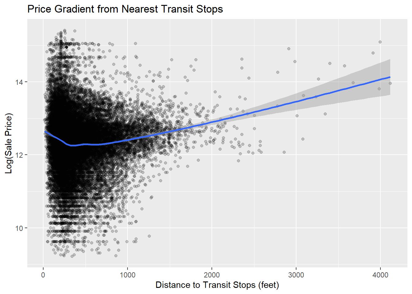
# Transit data on SEPTA bus/subways stops and regional rail stations: https://opendataphilly.org/datasets/septa-routes-stops-locations/
stops <- st_read("data/Transit_Stops_(Spring_2025)/Transit_Stops_(Spring_2025).shp")

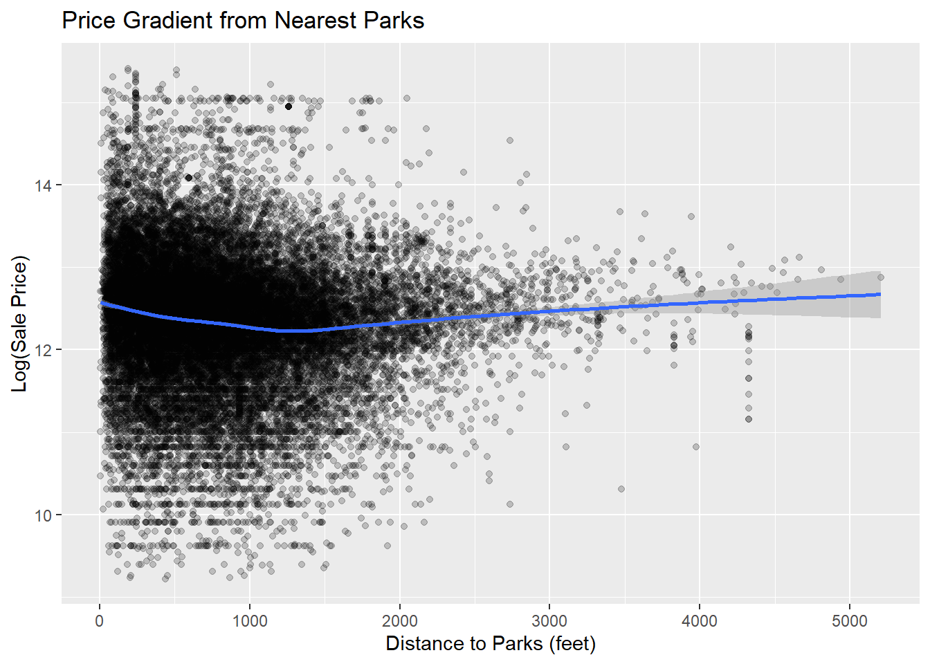
# Parks/Green Space: https://opendataphilly.org/datasets/ppr-properties/
parks <- st_read("data/PPR_Properties/PPR_Properties.shp")

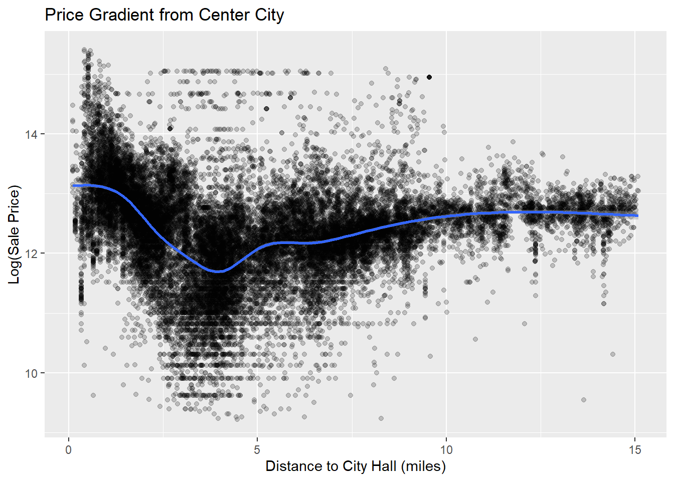
# Distance to Center City (anchor to city hall)
city_hall <- st_as_sf(
  data.frame(
    name = "City Hall",
    lon = -75.1636,
    lat = 39.9526
  ),
  coords = c("lon", "lat"),
  crs = 4326
)

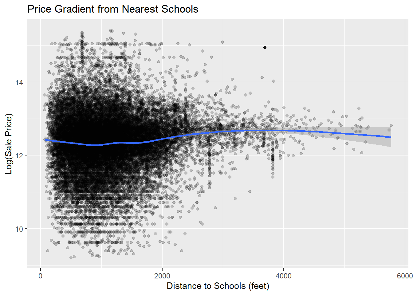
# Schools: https://opendataphilly.org/datasets/schools/
schools <- st_read("data/Schools/Schools.shp")

# Crime: https://opendataphilly.org/datasets/crime-incidents/
crime <- st_read("data/incidents_part1_part2/incidents_part1_part2.shp")

# Crashes: https://opendataphilly.org/datasets/crashes/
crash <- st_read("data/collision_crash_2020_2024/collision_crash_2020_2024.shp")

# Landmarks: https://opendataphilly.org/datasets/city-landmarks/
landmarks <- st_read("data/Landmark_Points/Landmark_Points.shp")

# PA Hospitals: https://opendataphilly.org/datasets/pa-hospitals/
hospitals <- st_read("data/DOH_Hospitals202311.geojson")

# Neighborhoods: https://opendataphilly.org/datasets/philadelphia-neighborhoods/
nb <- st_read("data/philadelphia-neighborhoods/philadelphia-neighborhoods.shp")

# Convert sales data to sf
sales_sf <- st_as_sf(
  sales_clean,
  coords = c("longitude", "latitude"),
  crs = 4326
)

# Match CRS to NAD83 Pennsylvania South (feet), 2272
sales_sf <- st_transform(sales_sf, 2272)
phl_census_wide <- st_transform(phl_census_wide, 2272)
stops  <- st_transform(stops, 2272)
parks  <- st_transform(parks, 2272)
city_hall <- st_transform(city_hall, 2272)
schools <- st_transform(schools, 2272)
crime <- st_transform(crime, 2272)
crash <- st_transform(crash, 2272)
landmarks <- st_transform(landmarks, 2272)
hospitals <- st_transform(hospitals, 2272)
nb <- st_transform(nb, 2272)

# Join census data to sales_clean
sales_sf <- st_join(sales_sf, phl_census_wide)
# Spatial join: Assign each house to its neighborhood
sales_sf <- sales_sf %>%
  st_join(nb, join = st_intersects)
  
# Check results
sales_sf %>%
  st_drop_geometry() %>%
  count(NAME) %>%
  arrange(desc(n))

Phase 2: Exploratory Data Analysis

Code
# 1 Distribution of sale prices (histogram)
ggplot(sales_sf, aes(x = sale_price)) +
  geom_histogram(bins = 50) +
  scale_x_continuous(labels = scales::dollar) +
  labs(
    title = "Distribution of Sale Prices (Raw)",
    x = "Sale Price",
    y = "Count"
  )

Code
# Log sale price
sales_sf <- sales_sf %>%
  mutate(
    log_price = log(sale_price)
  )

# 1 Distribution of log sale prices (histogram)
ggplot(sales_sf, aes(x = log_price)) +
  geom_histogram(bins = 50) +
  labs( 
    title = "Distribution of Log Sale Prices",
    x = "Log(Sale Price)",
    y = "Count"
  )

Interpretation: Raw prices are heavily right-skewed, meaning there are a lot of expensive outliers in our housing sale price data. Log transformation produces a more symmetric distribution suitable for regression modeling.

Code
# 2 Geographic distribution (map)
ggplot(sales_sf) +
  geom_sf(aes(color = log_price)) +
  scale_color_viridis_c() +
  labs(title = "Spatial Distribution of Home Prices (Log Scale)")+
  theme_minimal()

Interpretation: Home prices exhibit strong spatial clustering across Philadelphia.Higher-priced properties concentrate in Center City and Northwest neighborhoods, while lower-priced homes are more prevalent in North and West Philadelphia.

Code
# 3 Price v. structural features (scatter plots)
# 3 Price v. total livable area
ggplot(sales_sf, aes(total_livable_area, log_price)) +
  geom_point(alpha = 0.2) +
  geom_smooth(method = "loess") +
  labs(
    title = "Sale Price vs. Living Area",
    x = "Living Area (sq ft)",
    y = "Log(Sale Price)"
  )
`geom_smooth()` using formula = 'y ~ x'

Code
# 4 Price v. spatial feature (scatter plots)
# 4 Price v. distance to downtown
sales_sf <- sales_sf %>%
  mutate(
    dist_downtown_ft = as.numeric(st_distance(geometry, city_hall)),
    dist_downtown_mi = dist_downtown_ft / 5280
  ) # Calculate distance to city hall

ggplot(sales_sf, aes(dist_downtown_mi, log_price)) +
  geom_point(alpha = 0.2) +
  geom_smooth() +
  labs(
    title = "Price Gradient from Center City",
    x = "Distance to City Hall (miles)",
    y = "Log(Sale Price)"
  )
`geom_smooth()` using method = 'gam' and formula = 'y ~ s(x, bs = "cs")'
Warning: Removed 2 rows containing non-finite outside the scale range
(`stat_smooth()`).
Warning: Removed 2 rows containing missing values or values outside the scale range
(`geom_point()`).

Interpretation: The relationship between distance to City Hall and log sale price is nonlinear. Prices decline sharply within the first 2-4 miles from city hall, but begin to recover in outer neighborhoods.

Code
# 4 Price v. spatial features (scatter plots)
# 4 Price v. distance to transit stops
stops_dist <- st_distance(sales_sf, stops) # Calculate distance to transit stops

get_knn_distance <- function(stops_dist, k) {
  apply(stops_dist, 1, function(distances){
    mean(as.numeric(sort(distances)[1:k]))
  })
} # Create function

sales_sf <- sales_sf %>%
  mutate(
    stops_nn1 = get_knn_distance(stops_dist, k= 1),
    stops_nn3 = get_knn_distance(stops_dist, k= 3),
    stops_nn5 = get_knn_distance(stops_dist, k= 5)
  ) # Create features

ggplot(sales_sf, aes(stops_nn1, log_price)) +
  geom_point(alpha = 0.2) +
  geom_smooth() +
  labs(
    title = "Price Gradient from Nearest Transit Stops",
    x = "Distance to Transit Stops (feet)",
    y = "Log(Sale Price)"
  )
`geom_smooth()` using method = 'gam' and formula = 'y ~ s(x, bs = "cs")'
Warning: Removed 2 rows containing non-finite outside the scale range
(`stat_smooth()`).
Warning: Removed 2 rows containing missing values or values outside the scale range
(`geom_point()`).

Interpretation: The relationship between distance to the nearest transit stop and sale price is nonlinear. Properties located extremely close to transit exhibit slightly lower prices, potentially reflecting noise or traffic externalities. Prices increase within a moderate walking distance range (500-1500ft), suggesting an accessibility premium. The relationship becomes unstable beyond 2000 ft due to limited observations.

Code
# 4 Price v. distance to schools
schools_dist <- st_distance(sales_sf, schools) # Calculate distance to schools

get_knn_distance <- function(schools_dist, k) {
  apply(schools_dist, 1, function(distances){
    mean(as.numeric(sort(distances)[1:k]))
  })
} # Create function

sales_sf <- sales_sf %>%
  mutate(
    schools_nn1 = get_knn_distance(schools_dist, k= 1),
    schools_nn3 = get_knn_distance(schools_dist, k= 3),
    schools_nn5 = get_knn_distance(schools_dist, k= 5)
  ) # Create features

ggplot(sales_sf, aes(schools_nn1, log_price)) +
  geom_point(alpha = 0.2) +
  geom_smooth() +
  labs(
    title = "Price Gradient from Nearest Schools",
    x = "Distance to Schools (feet)",
    y = "Log(Sale Price)"
  )
`geom_smooth()` using method = 'gam' and formula = 'y ~ s(x, bs = "cs")'
Warning: Removed 2 rows containing non-finite outside the scale range
(`stat_smooth()`).
Warning: Removed 2 rows containing missing values or values outside the scale range
(`geom_point()`).

Interpretation: The relationship between distance to the nearest schools and sale price is relatively weak and nonlinear. Properties immediately adjacent to schools do not exhibit a strong premium. Moderate proximity (2000-4000ft) is associated with slightly higher prices.

Code
# 4 Price v. distance to parks
parks_dist <- st_distance(sales_sf, parks) # Calculate distance to parks

get_knn_distance <- function(parks_dist, k) {
  apply(parks_dist, 1, function(distances){
    mean(as.numeric(sort(distances)[1:k]))
  })
} # Create function

sales_sf <- sales_sf %>%
  mutate(
    parks_nn1 = get_knn_distance(parks_dist, k= 1),
    parks_nn3 = get_knn_distance(parks_dist, k= 3),
    parks_nn5 = get_knn_distance(parks_dist, k= 5)
  ) # Create features

ggplot(sales_sf, aes(parks_nn1, log_price)) +
  geom_point(alpha = 0.2) +
  geom_smooth() +
  labs(
    title = "Price Gradient from Nearest Parks",
    x = "Distance to Parks (feet)",
    y = "Log(Sale Price)"
  )
`geom_smooth()` using method = 'gam' and formula = 'y ~ s(x, bs = "cs")'
Warning: Removed 2 rows containing non-finite outside the scale range
(`stat_smooth()`).
Warning: Removed 2 rows containing missing values or values outside the scale range
(`geom_point()`).

Interpretation: The relationship between distance to the nearest park and sale price is weak and nonlinear. Properties immediately adjacent to parks show a small premium, but the advantage flattens quickly beyond 1000ft. This suggests that park proximity may confer localized amenity benefits, but its explanatory power to sale price is limited to external factors.

Code
# 5 Price by income quantile
sales_sf %>%
  filter(!is.na(med_income)) %>%   # drop NA
  mutate(
    income_q = ntile(med_income, 4),
    income_q = factor(
      income_q,
      levels = 1:4,
      labels = c(
        "Lowest Income",
        "Lower-Middle",
        "Upper-Middle",
        "Highest Income"
      )
    )
  ) %>%
  ggplot(aes(income_q, log_price)) +
  geom_boxplot(fill = "steelblue", alpha = 0.6) +
  labs(
    title = "Home Prices by Neighborhood Income Quartile",
    x = "Income Quartile",
    y = "Log(Sale Price)"
  ) +
  theme_minimal()

Interpretation: Sale prices increase monotonically across neighborhood income quartiles. The median log sale price in the highest-income quartile is substantially higher than in the lowest-income quartile, indicating strong neighborhood-level stratification in the housing market.

Code
# 5 Price by neighborhood
neighborhood_price <- sales_sf %>%
  st_drop_geometry() %>%
  group_by(NAME) %>%
  summarise(
    median_price = median(sale_price, na.rm = TRUE)
  ) # Calculate median price by neighborhood

nb_map <- nb %>%
  left_join(neighborhood_price, by = "NAME") # Sptial join

ggplot(nb_map) +
  geom_sf(aes(fill = median_price), color = "white", linewidth = 0.3) +
  scale_fill_viridis_c(labels = scales::dollar) +
  labs(
    title = "Median Sale Price by Neighborhood",
    fill = "Median Price"
  ) +
  theme_minimal()

Phase 3: Feature Engineering (Technical Appendix)

Code
#buffer-based
# number of parks/schools/transit stops within 0.25 or 0.5 or 1 or 2 miles
# crime
# car crashes
# hospitals
# monuments

#census variables
# income
# education
# poverty
# owner occ
# % rent burden

#interaction terms
# does crime rate matter more in low-income neighborhoods (or high-income) -- potential for price to drop in
#     high-income is higher, but low-income may be penalized more for frequency?
# distance to park * income (might be less or more of an incentive in low-income neighborhoods)
# distance to CC * # of transit stops -- less important for ppl far away from center city?
# distance to landmarks * sqf -- more premium in historically sig areas
# distance to city hall * sqf -- sqf values more in central areas
# built year * sqf -- sqf values more in the modern and the most historic homes

# 0.5 miles -- 10 mins walking
# 0.25 miles -- 5 mins walking

#BUFFER-BASED
# Flag homes with number of parks within 2 miles
# Parks provide recreational space, environmental quality, and aesthetic value, which can increase nearby property desirability and housing prices.
sales_sf <- sales_sf %>%
  mutate(
    parks_2m = lengths(st_intersects(
      st_buffer(geometry, 10560),
      parks)),
    parks_1m = lengths(st_intersects(
      st_buffer(geometry, 5280),
      parks)),
    parks_05m = lengths(st_intersects(
      st_buffer(geometry, 2640),
      parks)),
    parks_025m = lengths(st_intersects(
      st_buffer(geometry, 1320),
      parks))
  )

# Calculate distance from each house to nearest park
nearest_index <- st_nearest_feature(sales_sf, parks)
nearest_dist <- st_distance(sales_sf, parks[nearest_index,],
                            by_element = TRUE)
sales_sf$nearest_park <- as.numeric(nearest_dist/5280) #make it in miles

# Flag homes with number of transit stops within 0.25 miles
# Proximity to transit improves accessibility to jobs and services, often increasing property values within walkable distance.
sales_sf <- sales_sf %>%
  mutate(
    transit_025m = lengths(st_intersects(
      st_buffer(geometry, 1320),
      stops
      ))
  )

# Flag homes with number of schools within 2 miles
# Access to schools is a key factor for households, especially families, and is often associated with higher housing demand and prices.
sales_sf <- sales_sf %>%
  mutate(
    schools_2m = lengths(st_intersects(
      st_buffer(geometry, 10560),
      schools
      ))
  )

# Flag homes with number of crime incidents within 0.25 miles
# Higher crime levels reduce perceived safety and neighborhood desirability, typically leading to lower property values.
sales_sf <- sales_sf %>%
  mutate(
    crime_025m = lengths(st_intersects(
      st_buffer(geometry, 1320),
      crime
      ))
  )

# Flag homes with number of car crashes within 0.25 miles
# High crash density may indicate traffic congestion and unsafe street conditions, negatively affecting residential desirability.
sales_sf <- sales_sf %>%
  mutate(
    crash_025m = lengths(st_intersects(
      st_buffer(geometry, 1320),
      crash
      ))
  )

# Flag homes with number of hospitals within 2 miles
# Proximity to healthcare facilities improves accessibility to essential services, though effects may vary depending on noise and traffic.
sales_sf <- sales_sf %>%
  mutate(
    hospitals_2m = lengths(st_intersects(
      st_buffer(geometry, 10560),
      hospitals
      ))
  )

# Flag homes with number of landmarks within 0.5 miles
# Cultural and historic landmarks enhance neighborhood identity and attractiveness, potentially increasing nearby property values.
sales_sf <- sales_sf %>%
  mutate(
    landmarks_05m = lengths(st_intersects(
      st_buffer(geometry, 2640),
      landmarks
      ))
  )

### Ultimately not used -- commented off for the sake of running the program
# # Create Missing KNN (landmarks, crashes, crimes, hospitals)
# landmarks_dist <- st_distance(sales_sf, landmarks) # Calculate distance to landmarks
# get_knn_distance <- function(landmarks_dist, k) {
#   apply(landmarks_dist, 1, function(distances){
#     mean(as.numeric(sort(distances)[1:k]))
#   })
# } # Create function
# sales_sf <- sales_sf %>%
#   mutate(
#     landmarks_nn1 = get_knn_distance(landmarks_dist, k= 1),
#     landmarks_nn3 = get_knn_distance(landmarks_dist, k= 3),
#     landmarks_nn5 = get_knn_distance(landmarks_dist, k= 5)
#   ) # Create feature
# 
# crash_dist <- st_distance(sales_sf, crash) # Calculate distance to car crashes
# get_knn_distance <- function(crash_dist, k) {
#   apply(crash_dist, 1, function(distances){
#     mean(as.numeric(sort(distances)[1:k]))
#   })
# } # Create function
# sales_sf <- sales_sf %>%
#   mutate(
#     crash_nn1 = get_knn_distance(crash_dist, k= 1),
#     crash_nn3 = get_knn_distance(crash_dist, k= 3),
#     crash_nn5 = get_knn_distance(crash_dist, k= 5)
#   ) # Create feature
# 
# crime_dist <- st_distance(sales_sf, crime) # Calculate distance to crimes
# get_knn_distance <- function(crime_dist, k) {
#   apply(crime_dist, 1, function(distances){
#     mean(as.numeric(sort(distances)[1:k]))
#   })
# } # Create function
# sales_sf <- sales_sf %>%
#   mutate(
#     crime_nn1 = get_knn_distance(crime_dist, k= 1),
#     crime_nn3 = get_knn_distance(crime_dist, k= 3),
#     crime_nn5 = get_knn_distance(crime_dist, k= 5)
#   ) # Create feature

# Create wealth dummy variable
sales_sf <- sales_sf %>%
  mutate(wealth = case_when(
    med_income < 45000 ~ "low",
    med_income > 90000 ~ "high",
    TRUE ~ "medium"
  ))
# Create age variable
sales_sf <- sales_sf %>%
  mutate(
    age = 2026 - as.numeric(year_built)
  )
# Neighborhood fixed effect
# Ensure name is a factor (i.e., categorical variable)
sales_sf <- sales_sf %>%
  mutate(NAME = as.factor(NAME))

# Check which is reference (first alphabetically)
levels(sales_sf$NAME)[1]
[1] "ACADEMY_GARDENS"
Code
###Commented off to ensure program runs, but used to determine which variable impacts sales price the most
# # Check which variable has the most impact on sales price
# sales_sf %>%
#   st_drop_geometry() %>%
#   select(sale_price, stops_nn1, stops_nn3, stops_nn5, transit_025m) %>%
#   cor(use = "complete.obs") %>%
#   as.data.frame() %>%
#   select(sale_price)
# cat("transit_025m has the largest coorelation with sale_price")
# 
# sales_sf %>%
#   st_drop_geometry() %>%
#   select(sale_price, schools_nn1, schools_nn3, schools_nn5, schools_2m) %>%
#   cor(use = "complete.obs") %>%
#   as.data.frame() %>%
#   select(sale_price)
# cat("schools_2m has the largest coorelation with sale_price")
# 
# sales_sf %>%
#   st_drop_geometry() %>%
#   select(sale_price, parks_nn1, parks_nn3, parks_nn5, parks_2m, parks_025m, parks_05m, parks_1m, nearest_park) %>%
#   cor(use = "complete.obs") %>%
#   as.data.frame() %>%
#   select(sale_price)
# cat("park_1m has the largest coorelation with sale_price")
# 
# sales_sf %>%
#   st_drop_geometry() %>%
#   select(sale_price, landmarks_nn1, landmarks_nn3, landmarks_nn5, landmarks_05m) %>%
#   cor(use = "complete.obs") %>%
#   as.data.frame() %>%
#   select(sale_price)
# cat("landmarks_05m has the largest coorelation with sale_price")
# 
# sales_sf %>%
#   st_drop_geometry() %>%
#   select(sale_price, crash_nn1, crash_nn3, crash_nn5, crash_025m) %>%
#   cor(use = "complete.obs") %>%
#   as.data.frame() %>%
#   select(sale_price)
# cat("crash_025m has the largest coorelation with sale_price")

# Population Density
sales_sf <- sales_sf %>%
  mutate(pop_density = total_pop/Shape_Area)

# Log sale price
sales_sf <- sales_sf %>%
  mutate(log_sale_price = log(sale_price))

Phase 4: Model Building

Build models progressively:

  1. Structural features only
    • Census variables
    • Spatial features
    • Interactions and fixed effects
Code
# Structural features only
# model1 <- lm(formula = sale_price ~ total_livable_area, data = sales_sf)
# summary(model1)
model2 <- lm(formula = log_sale_price ~ total_livable_area + number_of_bathrooms + number_of_bedrooms + number_stories + age, data = sales_sf)
summary(model2)

Call:
lm(formula = log_sale_price ~ total_livable_area + number_of_bathrooms + 
    number_of_bedrooms + number_stories + age, data = sales_sf)

Residuals:
    Min      1Q  Median      3Q     Max 
-4.8607 -0.3204  0.0752  0.3864  3.3977 

Coefficients:
                      Estimate Std. Error t value Pr(>|t|)    
(Intercept)          1.177e+01  1.990e-02  591.72  < 2e-16 ***
total_livable_area   4.636e-04  9.219e-06   50.29  < 2e-16 ***
number_of_bathrooms  4.025e-01  7.477e-03   53.83  < 2e-16 ***
number_of_bedrooms  -1.549e-01  5.316e-03  -29.14  < 2e-16 ***
number_stories       2.313e-02  8.383e-03    2.76  0.00579 ** 
age                 -2.523e-03  1.214e-04  -20.79  < 2e-16 ***
---
Signif. codes:  0 '***' 0.001 '**' 0.01 '*' 0.05 '.' 0.1 ' ' 1

Residual standard error: 0.6816 on 25255 degrees of freedom
Multiple R-squared:  0.3221,    Adjusted R-squared:  0.3219 
F-statistic:  2400 on 5 and 25255 DF,  p-value: < 2.2e-16
Code
# + Census variables
# model3 <- lm(formula = sale_price ~ total_livable_area + number_of_bathrooms + number_of_bedrooms + number_stories + age #structural
# + med_income + pct_college + poverty_rate + pct_owner_occ #census
# , data = sales_sf)
# summary(model3)
model3_2 <- lm(formula = log_sale_price ~ total_livable_area + number_of_bathrooms + number_of_bedrooms + number_stories + age #structural
+ med_income + pct_college + poverty_rate + pct_owner_occ 
+ pct_rent_burden + white + black + latinx + car + transit + remote + pop_density #census
, data = sales_sf)
summary(model3_2)

Call:
lm(formula = log_sale_price ~ total_livable_area + number_of_bathrooms + 
    number_of_bedrooms + number_stories + age + med_income + 
    pct_college + poverty_rate + pct_owner_occ + pct_rent_burden + 
    white + black + latinx + car + transit + remote + pop_density, 
    data = sales_sf)

Residuals:
    Min      1Q  Median      3Q     Max 
-3.9180 -0.2235  0.0452  0.2538  3.6174 

Coefficients:
                      Estimate Std. Error t value Pr(>|t|)    
(Intercept)          1.241e+01  7.021e-02 176.798  < 2e-16 ***
total_livable_area   3.092e-04  7.686e-06  40.228  < 2e-16 ***
number_of_bathrooms  1.931e-01  6.399e-03  30.182  < 2e-16 ***
number_of_bedrooms   2.684e-02  4.698e-03   5.713 1.12e-08 ***
number_stories       1.973e-02  6.934e-03   2.845  0.00444 ** 
age                 -1.698e-03  1.013e-04 -16.764  < 2e-16 ***
med_income           1.123e-06  2.822e-07   3.979 6.93e-05 ***
pct_college          7.429e-01  4.175e-02  17.796  < 2e-16 ***
poverty_rate        -4.899e-01  4.966e-02  -9.866  < 2e-16 ***
pct_owner_occ        1.086e-01  3.631e-02   2.992  0.00277 ** 
pct_rent_burden      1.991e-01  1.247e-01   1.597  0.11037    
white               -2.723e-01  4.297e-02  -6.337 2.39e-10 ***
black               -7.662e-01  3.702e-02 -20.698  < 2e-16 ***
latinx              -8.928e-01  4.173e-02 -21.392  < 2e-16 ***
car                 -4.940e-01  4.952e-02  -9.975  < 2e-16 ***
transit             -8.780e-01  6.720e-02 -13.065  < 2e-16 ***
remote              -7.354e-01  7.201e-02 -10.213  < 2e-16 ***
pop_density          1.870e+01  1.335e+01   1.401  0.16136    
---
Signif. codes:  0 '***' 0.001 '**' 0.01 '*' 0.05 '.' 0.1 ' ' 1

Residual standard error: 0.5428 on 24476 degrees of freedom
  (767 observations deleted due to missingness)
Multiple R-squared:  0.5566,    Adjusted R-squared:  0.5563 
F-statistic:  1808 on 17 and 24476 DF,  p-value: < 2.2e-16
Code
# + Spatial features
model4 <- lm(formula = log_sale_price ~ total_livable_area + number_of_bathrooms + number_of_bedrooms + number_stories + age #structural
+ med_income + pct_college + poverty_rate + pct_owner_occ 
+ pct_rent_burden + white + black + latinx + car + transit + remote + pop_density #census
+ parks_2m + transit_025m + schools_2m + crime_025m + crash_025m + hospitals_2m + landmarks_05m #spatial
, data = sales_sf)
summary(model4)

Call:
lm(formula = log_sale_price ~ total_livable_area + number_of_bathrooms + 
    number_of_bedrooms + number_stories + age + med_income + 
    pct_college + poverty_rate + pct_owner_occ + pct_rent_burden + 
    white + black + latinx + car + transit + remote + pop_density + 
    parks_2m + transit_025m + schools_2m + crime_025m + crash_025m + 
    hospitals_2m + landmarks_05m, data = sales_sf)

Residuals:
    Min      1Q  Median      3Q     Max 
-3.9543 -0.2223  0.0442  0.2495  3.6178 

Coefficients:
                      Estimate Std. Error t value Pr(>|t|)    
(Intercept)          1.274e+01  7.955e-02 160.112  < 2e-16 ***
total_livable_area   2.995e-04  7.712e-06  38.839  < 2e-16 ***
number_of_bathrooms  1.951e-01  6.390e-03  30.532  < 2e-16 ***
number_of_bedrooms   2.697e-02  4.729e-03   5.703 1.19e-08 ***
number_stories       3.274e-02  7.113e-03   4.602 4.20e-06 ***
age                 -1.618e-03  1.016e-04 -15.927  < 2e-16 ***
med_income           1.424e-06  2.846e-07   5.004 5.65e-07 ***
pct_college          6.493e-01  4.409e-02  14.726  < 2e-16 ***
poverty_rate        -4.165e-01  5.036e-02  -8.270  < 2e-16 ***
pct_owner_occ        5.999e-02  3.719e-02   1.613 0.106807    
pct_rent_burden      2.142e-01  1.293e-01   1.657 0.097507 .  
white               -2.997e-01  4.401e-02  -6.809 1.01e-11 ***
black               -7.434e-01  3.788e-02 -19.623  < 2e-16 ***
latinx              -8.269e-01  4.494e-02 -18.399  < 2e-16 ***
car                 -7.621e-01  6.032e-02 -12.634  < 2e-16 ***
transit             -9.461e-01  7.186e-02 -13.166  < 2e-16 ***
remote              -8.529e-01  7.539e-02 -11.312  < 2e-16 ***
pop_density          3.077e+01  1.362e+01   2.259 0.023913 *  
parks_2m            -1.115e-03  3.752e-04  -2.971 0.002970 ** 
transit_025m        -6.865e-04  2.144e-04  -3.202 0.001366 ** 
schools_2m          -9.029e-04  3.761e-04  -2.401 0.016377 *  
crime_025m          -6.291e-05  1.911e-05  -3.292 0.000997 ***
crash_025m          -5.558e-04  1.157e-04  -4.804 1.56e-06 ***
hospitals_2m         5.221e-03  2.783e-03   1.876 0.060675 .  
landmarks_05m        3.913e-03  4.658e-04   8.401  < 2e-16 ***
---
Signif. codes:  0 '***' 0.001 '**' 0.01 '*' 0.05 '.' 0.1 ' ' 1

Residual standard error: 0.5405 on 24469 degrees of freedom
  (767 observations deleted due to missingness)
Multiple R-squared:  0.5605,    Adjusted R-squared:  0.5601 
F-statistic:  1300 on 24 and 24469 DF,  p-value: < 2.2e-16
Code
# Interactions + fixed effects
# model5 <- lm(formula = sale_price ~ total_livable_area + number_of_bathrooms + number_of_bedrooms + number_stories + age #structural
# + med_income + pct_college + poverty_rate + pct_owner_occ 
# + pct_rent_burden + white + black + latinx + car + transit + remote + pop_density#census
# + parks_2m + transit_025m + schools_2m + crime_025m + crash_025m + hospitals_2m + landmarks_05m #spatial
# + NAME
# , data = sales_sf)
# summary(model5)

# 2
# Interactions + fixed effects
# does crime rate matter more in low-income neighborhoods (or high-income) -- potential for price to drop in
#     high-income is higher, but low-income may be penalized more for frequency?
# distance to park * income (might be less or more of an incentive in low-income neighborhoods)
# distance to CC * # of transit stops -- less important for ppl far away from center city?
# distance to landmarks * sqf -- more premium in historically sig areas
# distance to city hall * sqf -- sqf values more in central areas
# built year * sqf -- sqf values more in the modern and the most historic homes

# model5_2 <- lm(formula = sale_price ~ total_livable_area + number_of_bathrooms + number_of_bedrooms + number_stories + age #structural
# + med_income + pct_college + poverty_rate + pct_owner_occ 
# + pct_rent_burden + white + black + latinx + car + transit + remote + pop_density#census
# + parks_2m + transit_025m + schools_2m + crime_025m + crash_025m + hospitals_2m + landmarks_05m #spatial
# + NAME #fixedeffect
# + crime_025m*med_income #interaction
# , data = sales_sf)
# summary(model5_2)
# 
# model5_3 <- lm(formula = sale_price ~ total_livable_area + number_of_bathrooms + number_of_bedrooms + number_stories + age #structural
# + med_income + pct_college + poverty_rate + pct_owner_occ 
# + pct_rent_burden + white + black + latinx + car + transit + remote + pop_density#census
# + parks_2m + transit_025m + schools_2m + crime_025m + crash_025m + hospitals_2m + landmarks_05m #spatial
# + NAME #fixedeffect
# + parks_2m*med_income #interaction
# , data = sales_sf)
# summary(model5_3)
# 
# model5_4 <- lm(formula = sale_price ~ total_livable_area + number_of_bathrooms + number_of_bedrooms + number_stories + age #structural
# + med_income + pct_college + poverty_rate + pct_owner_occ 
# + pct_rent_burden + white + black + latinx + car + transit + remote + pop_density#census
# + parks_2m + transit_025m + schools_2m + crime_025m + crash_025m + hospitals_2m + landmarks_05m #spatial
# + NAME #fixedeffect
# + dist_downtown_mi*transit_025m #interaction
# , data = sales_sf)
# summary(model5_4)
# 
# model5_5 <- lm(formula = sale_price ~ total_livable_area + number_of_bathrooms + number_of_bedrooms + number_stories + age #structural
# + med_income + pct_college + poverty_rate + pct_owner_occ 
# + pct_rent_burden + white + black + latinx + car + transit + remote + pop_density#census
# + parks_2m + transit_025m + schools_2m + crime_025m + crash_025m + hospitals_2m + landmarks_05m #spatial
# + NAME #fixedeffect
# + landmarks_05m*total_livable_area #interaction
# , data = sales_sf)
# summary(model5_5)
# #0.4736
# 
# model5_6 <- lm(formula = sale_price ~ total_livable_area + number_of_bathrooms + number_of_bedrooms + number_stories + age #structural
# + med_income + pct_college + poverty_rate + pct_owner_occ 
# + pct_rent_burden + white + black + latinx + car + transit + remote + pop_density#census
# + parks_2m + transit_025m + schools_2m + crime_025m + crash_025m + hospitals_2m + landmarks_05m #spatial
# + NAME #fixedeffect
# + dist_downtown_mi*total_livable_area #interaction
# , data = sales_sf)
# summary(model5_6)
# #0.436
# 
# model5_7 <- lm(formula = sale_price ~ total_livable_area + number_of_bathrooms + number_of_bedrooms + number_stories + age #structural
# + med_income + pct_college + poverty_rate + pct_owner_occ 
# + pct_rent_burden + white + black + latinx + car + transit + remote + pop_density#census
# + parks_2m + transit_025m + schools_2m + crime_025m + crash_025m + hospitals_2m + landmarks_05m #spatial
# + NAME #fixedeffect
# + age*total_livable_area #interaction
# , data = sales_sf)
# summary(model5_7)
# 
# model5_8 <- lm(formula = sale_price ~ total_livable_area + number_of_bathrooms + number_of_bedrooms + number_stories + age #structural
# + med_income + pct_college + poverty_rate + pct_owner_occ 
# + pct_rent_burden + white + black + latinx + car + transit + remote + pop_density#census
# + parks_2m + transit_025m + schools_2m + crime_025m + crash_025m + hospitals_2m + landmarks_05m #spatial
# + NAME #fixedeffect
# + landmarks_05m*total_livable_area
# + dist_downtown_mi*transit_025m #interaction
# , data = sales_sf)
# summary(model5_8)
# 
# model6_2 <- lm(formula = sale_price ~ total_livable_area + number_of_bathrooms + number_of_bedrooms + number_stories + age #structural
# + med_income + pct_college + poverty_rate + pct_owner_occ 
# + pct_rent_burden + white + black + latinx + car + transit + remote + pop_density#census
# + parks_2m + transit_025m + schools_2m + crime_025m + crash_025m + hospitals_2m + landmarks_05m #spatial
# + NAME #fixedeffect
# + landmarks_05m*total_livable_area
# + dist_downtown_mi*transit_025m #interaction
# + I(age^2)
# , data = sales_sf)
# summary(model6_2)
# #0.471
# 
# model6_3 <- lm(formula = sale_price ~ total_livable_area + number_of_bathrooms + number_of_bedrooms + number_stories + age #structural
# + med_income + pct_college + poverty_rate + pct_owner_occ 
# + pct_rent_burden + white + black + latinx + car + transit + remote + pop_density#census
# + parks_2m + transit_025m + schools_2m + crime_025m + crash_025m + hospitals_2m + landmarks_05m #spatial
# + NAME #fixedeffect
# + landmarks_05m*total_livable_area
# + dist_downtown_mi*transit_025m #interaction
# + dist_downtown_mi + I(dist_downtown_mi^2)
# , data = sales_sf)
# summary(model6_3)
# #0.4704
# 
# model6_4 <- lm(formula = sale_price ~ total_livable_area + number_of_bathrooms + number_of_bedrooms + number_stories + age #structural
# + med_income + pct_college + poverty_rate + pct_owner_occ 
# + pct_rent_burden + white + black + latinx + car + transit + remote + pop_density#census
# + parks_2m + transit_025m + schools_2m + crime_025m + crash_025m + hospitals_2m + landmarks_05m #spatial
# + NAME #fixed effect
# + landmarks_05m*total_livable_area
# + dist_downtown_mi*transit_025m #interaction
# + I(age^2)
# , data = sales_sf)
# summary(model6_4)
# #0.471
# 
# model6_5 <- lm(formula = sale_price ~ total_livable_area + number_of_bathrooms + number_of_bedrooms + age #structural
# + med_income + pct_college + poverty_rate + pct_owner_occ 
# + pct_rent_burden + white + black + latinx + car + transit + remote + pop_density#census
# + parks_2m + transit_025m + schools_2m + crime_025m + crash_025m + hospitals_2m + landmarks_05m #spatial
# + NAME #fixedeffect
# + crime_025m*med_income
# + parks_2m*med_income
# + landmarks_05m*total_livable_area
# + dist_downtown_mi*transit_025m
# + dist_downtown_mi*total_livable_area 
# + age*total_livable_area #interaction
# + pct_owner_occ*total_livable_area
# + number_stories*med_income
# + I(age^2)
# + dist_downtown_mi + I(dist_downtown_mi^2)
# , data = sales_sf)
# summary(model6_5)
# #0.4763

##FINAL###
model6_5 <- lm(formula = log_sale_price ~ total_livable_area + number_of_bathrooms + age #structural
+ med_income + pct_college + poverty_rate + pct_owner_occ + white + black + car + transit + remote + pop_density #census
+ parks_2m + transit_025m + schools_2m + crime_025m + crash_025m + hospitals_2m + landmarks_05m #spatial
+ NAME #fixedeffect
+ crime_025m*med_income
+ parks_2m*med_income
+ landmarks_05m*total_livable_area
+ dist_downtown_mi*transit_025m
+ dist_downtown_mi*total_livable_area 
+ age*total_livable_area #interaction
+ pct_owner_occ*total_livable_area
+ pct_rent_burden*black
+ number_stories*med_income
+ I(age^2)
+ dist_downtown_mi + I(dist_downtown_mi^2)
, data = sales_sf)
summary(model6_5)

Call:
lm(formula = log_sale_price ~ total_livable_area + number_of_bathrooms + 
    age + med_income + pct_college + poverty_rate + pct_owner_occ + 
    white + black + car + transit + remote + pop_density + parks_2m + 
    transit_025m + schools_2m + crime_025m + crash_025m + hospitals_2m + 
    landmarks_05m + NAME + crime_025m * med_income + parks_2m * 
    med_income + landmarks_05m * total_livable_area + dist_downtown_mi * 
    transit_025m + dist_downtown_mi * total_livable_area + age * 
    total_livable_area + pct_owner_occ * total_livable_area + 
    pct_rent_burden * black + number_stories * med_income + I(age^2) + 
    dist_downtown_mi + I(dist_downtown_mi^2), data = sales_sf)

Residuals:
    Min      1Q  Median      3Q     Max 
-4.4053 -0.1972  0.0396  0.2248  3.7697 

Coefficients:
                                      Estimate Std. Error t value Pr(>|t|)    
(Intercept)                          1.159e+01  2.646e-01  43.779  < 2e-16 ***
total_livable_area                   3.578e-04  2.566e-05  13.947  < 2e-16 ***
number_of_bathrooms                  1.794e-01  5.785e-03  31.016  < 2e-16 ***
age                                 -1.909e-03  1.592e-04 -11.992  < 2e-16 ***
med_income                           8.071e-07  6.210e-07   1.300 0.193729    
pct_college                          2.632e-01  6.457e-02   4.076 4.59e-05 ***
poverty_rate                        -1.754e-03  5.943e-02  -0.030 0.976454    
pct_owner_occ                        1.840e-01  7.375e-02   2.495 0.012605 *  
white                                4.253e-01  5.070e-02   8.388  < 2e-16 ***
black                               -2.064e-01  5.422e-02  -3.807 0.000141 ***
car                                 -1.243e-01  8.357e-02  -1.487 0.137066    
transit                             -1.921e-01  9.137e-02  -2.102 0.035574 *  
remote                              -1.373e-01  1.020e-01  -1.345 0.178614    
pop_density                         -4.231e+01  5.312e+01  -0.797 0.425730    
parks_2m                             3.387e-03  1.177e-03   2.878 0.004005 ** 
transit_025m                        -4.885e-04  4.174e-04  -1.170 0.241876    
schools_2m                          -1.775e-03  9.265e-04  -1.915 0.055442 .  
crime_025m                          -1.022e-04  4.184e-05  -2.444 0.014548 *  
crash_025m                          -6.328e-04  1.394e-04  -4.539 5.68e-06 ***
hospitals_2m                        -2.133e-03  5.326e-03  -0.400 0.688847    
landmarks_05m                       -6.362e-03  1.085e-03  -5.863 4.61e-09 ***
NAMEALLEGHENY_WEST                  -2.923e-01  1.138e-01  -2.569 0.010210 *  
NAMEANDORRA                          7.969e-02  1.015e-01   0.785 0.432492    
NAMEASTON_WOODBRIDGE                 3.051e-02  8.731e-02   0.350 0.726705    
NAMEBARTRAM_VILLAGE                  6.293e-02  1.707e-01   0.369 0.712346    
NAMEBELLA_VISTA                      4.275e-01  1.507e-01   2.837 0.004556 ** 
NAMEBELMONT                         -9.011e-02  1.512e-01  -0.596 0.551148    
NAMEBREWERYTOWN                      1.173e-01  1.237e-01   0.948 0.343234    
NAMEBRIDESBURG                      -1.448e-01  1.036e-01  -1.397 0.162303    
NAMEBURHOLME                         2.699e-01  1.189e-01   2.269 0.023258 *  
NAMEBUSTLETON                        5.823e-02  6.224e-02   0.936 0.349530    
NAMEBYBERRY                          4.912e-03  1.595e-01   0.031 0.975434    
NAMECALLOWHILL                       3.938e-01  1.713e-01   2.300 0.021475 *  
NAMECARROLL_PARK                    -2.252e-02  1.170e-01  -0.192 0.847405    
NAMECEDAR_PARK                       4.845e-01  1.352e-01   3.583 0.000341 ***
NAMECEDARBROOK                       4.097e-01  9.254e-02   4.427 9.59e-06 ***
NAMECENTER_CITY                      8.037e-01  2.641e-01   3.043 0.002341 ** 
NAMECHESTNUT_HILL                    3.951e-01  8.983e-02   4.398 1.10e-05 ***
NAMECLEARVIEW                        2.046e-01  1.436e-01   1.425 0.154291    
NAMECOBBS_CREEK                      2.403e-01  1.183e-01   2.032 0.042213 *  
NAMECRESCENTVILLE                    2.589e-01  2.724e-01   0.950 0.341907    
NAMEDEARNLEY_PARK                   -1.648e-01  1.174e-01  -1.404 0.160382    
NAMEDICKINSON_NARROWS                2.525e-01  1.443e-01   1.749 0.080273 .  
NAMEDUNLAP                           1.872e-01  1.690e-01   1.107 0.268198    
NAMEEAST_FALLS                       3.627e-02  1.069e-01   0.339 0.734305    
NAMEEAST_KENSINGTON                  3.744e-01  1.252e-01   2.991 0.002784 ** 
NAMEEAST_OAK_LANE                    2.103e-01  1.047e-01   2.009 0.044566 *  
NAMEEAST_PARK                        4.863e-01  5.349e-01   0.909 0.363308    
NAMEEAST_PARKSIDE                   -2.443e-01  1.501e-01  -1.628 0.103583    
NAMEEAST_PASSYUNK                    4.015e-01  1.399e-01   2.869 0.004126 ** 
NAMEEAST_POPLAR                      4.358e-02  2.127e-01   0.205 0.837630    
NAMEEASTWICK                         3.981e-01  1.333e-01   2.986 0.002827 ** 
NAMEELMWOOD                         -6.307e-02  1.254e-01  -0.503 0.615123    
NAMEFAIRHILL                        -6.472e-01  1.311e-01  -4.937 7.99e-07 ***
NAMEFAIRMOUNT                        2.721e-01  1.343e-01   2.027 0.042684 *  
NAMEFELTONVILLE                     -1.625e-01  1.006e-01  -1.615 0.106360    
NAMEFERN_ROCK                        2.445e-01  1.250e-01   1.956 0.050520 .  
NAMEFISHTOWN                         2.211e-01  1.238e-01   1.787 0.073992 .  
NAMEFITLER_SQUARE                    6.757e-01  1.728e-01   3.911 9.22e-05 ***
NAMEFOX_CHASE                        9.308e-02  7.145e-02   1.303 0.192704    
NAMEFRANCISVILLE                     3.190e-01  1.402e-01   2.276 0.022856 *  
NAMEFRANKFORD                       -2.769e-01  9.118e-02  -3.037 0.002393 ** 
NAMEFRANKLINVILLE                   -4.956e-01  1.195e-01  -4.149 3.36e-05 ***
NAMEGARDEN_COURT                     5.818e-01  1.720e-01   3.382 0.000720 ***
NAMEGERMANTOWN_EAST                  4.821e-02  9.554e-02   0.505 0.613799    
NAMEGERMANTOWN_MORTON                9.582e-02  1.033e-01   0.928 0.353514    
NAMEGERMANTOWN_PENN_KNOX             1.674e-01  1.682e-01   0.995 0.319754    
NAMEGERMANTOWN_SOUTHWEST             5.461e-02  1.064e-01   0.514 0.607603    
NAMEGERMANTOWN_WEST_CENT             2.318e-01  1.193e-01   1.943 0.051983 .  
NAMEGERMANTOWN_WESTSIDE              1.067e-02  1.368e-01   0.078 0.937826    
NAMEGERMANY_HILL                     3.491e-02  1.121e-01   0.311 0.755469    
NAMEGIRARD_ESTATES                   1.508e-01  1.340e-01   1.126 0.260224    
NAMEGLENWOOD                        -4.862e-01  1.272e-01  -3.821 0.000133 ***
NAMEGRADUATE_HOSPITAL                4.694e-01  1.361e-01   3.450 0.000562 ***
NAMEGRAYS_FERRY                      6.652e-02  1.341e-01   0.496 0.619806    
NAMEGREENWICH                        3.941e-01  1.972e-01   1.998 0.045687 *  
NAMEHADDINGTON                      -9.238e-02  1.162e-01  -0.795 0.426542    
NAMEHARROWGATE                      -3.632e-01  1.142e-01  -3.179 0.001478 ** 
NAMEHARTRANFT                       -6.779e-01  1.200e-01  -5.649 1.63e-08 ***
NAMEHAVERFORD_NORTH                 -1.345e-01  1.679e-01  -0.801 0.423204    
NAMEHAWTHORNE                        4.530e-01  1.538e-01   2.945 0.003231 ** 
NAMEHOLMESBURG                      -2.606e-02  6.842e-02  -0.381 0.703243    
NAMEHUNTING_PARK                    -7.785e-02  1.062e-01  -0.733 0.463477    
NAMEJUNIATA_PARK                    -2.492e-02  1.012e-01  -0.246 0.805507    
NAMEKINGSESSING                      9.991e-02  1.242e-01   0.804 0.421338    
NAMELAWNDALE                         1.720e-01  8.658e-02   1.987 0.046961 *  
NAMELEXINGTON_PARK                   5.585e-01  8.977e-02   6.221 5.01e-10 ***
NAMELOGAN                            1.514e-01  1.031e-01   1.469 0.141875    
NAMELOGAN_SQUARE                     4.634e-01  1.463e-01   3.168 0.001538 ** 
NAMELOWER_MOYAMENSING                3.352e-02  1.334e-01   0.251 0.801532    
NAMELUDLOW                           1.251e-01  1.876e-01   0.667 0.504697    
NAMEMANAYUNK                         1.184e-04  9.886e-02   0.001 0.999044    
NAMEMANTUA                           9.172e-02  1.381e-01   0.664 0.506452    
NAMEMAYFAIR                          1.123e-01  7.441e-02   1.509 0.131380    
NAMEMCGUIRE                         -8.916e-01  1.415e-01  -6.302 2.98e-10 ***
NAMEMECHANICSVILLE                   1.224e-01  3.266e-01   0.375 0.707817    
NAMEMELROSE_PARK_GARDENS             2.439e-01  1.247e-01   1.956 0.050459 .  
NAMEMILL_CREEK                      -3.145e-01  1.249e-01  -2.518 0.011797 *  
NAMEMILLBROOK                       -4.992e-02  8.612e-02  -0.580 0.562104    
NAMEMODENA                          -1.293e-01  7.515e-02  -1.721 0.085321 .  
NAMEMORRELL_PARK                    -4.660e-02  7.169e-02  -0.650 0.515708    
NAMEMOUNT_AIRY_EAST                  2.989e-01  8.733e-02   3.423 0.000621 ***
NAMEMOUNT_AIRY_WEST                  2.150e-01  9.277e-02   2.317 0.020504 *  
NAMENEWBOLD                          2.506e-01  1.416e-01   1.769 0.076859 .  
NAMENICETOWN                        -1.865e-01  1.451e-01  -1.285 0.198748    
NAMENORMANDY_VILLAGE                -3.581e-03  1.407e-01  -0.025 0.979698    
NAMENORTH_CENTRAL                    7.302e-02  1.249e-01   0.584 0.558905    
NAMENORTHERN_LIBERTIES               2.557e-01  1.329e-01   1.924 0.054370 .  
NAMENORTHWOOD                        1.087e-01  9.943e-02   1.093 0.274325    
NAMEOGONTZ                           1.234e-01  9.423e-02   1.309 0.190440    
NAMEOLD_CITY                         4.158e-01  1.444e-01   2.879 0.003991 ** 
NAMEOLD_KENSINGTON                   2.150e-01  1.331e-01   1.616 0.106199    
NAMEOLNEY                            8.399e-03  9.366e-02   0.090 0.928542    
NAMEOVERBROOK                        1.287e-01  1.108e-01   1.162 0.245367    
NAMEOXFORD_CIRCLE                    1.377e-01  7.712e-02   1.786 0.074092 .  
NAMEPACKER_PARK                      1.963e-01  1.475e-01   1.330 0.183417    
NAMEPARKWOOD_MANOR                  -7.951e-02  8.938e-02  -0.890 0.373683    
NAMEPASCHALL                        -1.862e-01  1.233e-01  -1.510 0.131170    
NAMEPASSYUNK_SQUARE                  3.080e-01  1.392e-01   2.213 0.026891 *  
NAMEPENNSPORT                        2.037e-01  1.424e-01   1.430 0.152630    
NAMEPENNYPACK                        5.352e-02  6.916e-02   0.774 0.439083    
NAMEPENNYPACK_PARK                  -1.895e-01  5.238e-01  -0.362 0.717511    
NAMEPENNYPACK_WOODS                 -9.168e-02  1.106e-01  -0.829 0.407148    
NAMEPENROSE                          1.492e-01  1.415e-01   1.054 0.291714    
NAMEPOINT_BREEZE                     2.188e-01  1.308e-01   1.673 0.094393 .  
NAMEPOWELTON                         6.542e-02  2.649e-01   0.247 0.804924    
NAMEQUEEN_VILLAGE                    4.276e-01  1.450e-01   2.948 0.003197 ** 
NAMERHAWNHURST                       1.678e-01  7.031e-02   2.387 0.017003 *  
NAMERICHMOND                        -8.151e-02  1.134e-01  -0.719 0.472111    
NAMERITTENHOUSE                      6.275e-01  1.426e-01   4.401 1.08e-05 ***
NAMERIVERFRONT                       1.670e-01  1.608e-01   1.038 0.299054    
NAMEROXBOROUGH                       4.699e-02  9.666e-02   0.486 0.626860    
NAMEROXBOROUGH_PARK                  7.963e-03  1.346e-01   0.059 0.952818    
NAMESHARSWOOD                        1.147e-01  1.387e-01   0.827 0.408006    
NAMESOCIETY_HILL                     4.084e-01  1.464e-01   2.790 0.005275 ** 
NAMESOMERTON                         1.019e-02  8.485e-02   0.120 0.904441    
NAMESOUTHWEST_SCHUYLKILL            -7.911e-02  1.335e-01  -0.592 0.553591    
NAMESPRING_GARDEN                    1.501e-01  1.400e-01   1.072 0.283548    
NAMESPRUCE_HILL                      4.793e-01  1.438e-01   3.334 0.000859 ***
NAMESTADIUM_DISTRICT                 2.140e-01  1.413e-01   1.514 0.129992    
NAMESTANTON                         -1.363e-01  1.184e-01  -1.151 0.249852    
NAMESTRAWBERRY_MANSION              -5.233e-01  1.183e-01  -4.425 9.67e-06 ***
NAMESUMMERDALE                       9.866e-02  9.811e-02   1.006 0.314622    
NAMETACONY                          -6.972e-02  7.666e-02  -0.909 0.363112    
NAMETIOGA                           -3.100e-01  1.138e-01  -2.723 0.006470 ** 
NAMETORRESDALE                      -1.137e-01  6.560e-02  -1.733 0.083124 .  
NAMEUNIVERSITY_CITY                 -4.133e-01  3.301e-01  -1.252 0.210573    
NAMEUPPER_KENSINGTON                -3.841e-01  1.094e-01  -3.510 0.000449 ***
NAMEUPPER_ROXBOROUGH                 7.642e-02  8.732e-02   0.875 0.381479    
NAMEWALNUT_HILL                      4.307e-01  1.449e-01   2.973 0.002947 ** 
NAMEWASHINGTON_SQUARE                4.008e-01  1.495e-01   2.681 0.007338 ** 
NAMEWEST_KENSINGTON                 -8.484e-02  1.229e-01  -0.691 0.489881    
NAMEWEST_OAK_LANE                    2.730e-01  8.808e-02   3.100 0.001939 ** 
NAMEWEST_PARKSIDE                   -2.630e-01  2.587e-01  -1.017 0.309350    
NAMEWEST_PASSYUNK                    1.343e-01  1.384e-01   0.970 0.331899    
NAMEWEST_POPLAR                      3.013e-01  1.793e-01   1.681 0.092851 .  
NAMEWEST_POWELTON                    2.858e-01  1.544e-01   1.851 0.064150 .  
NAMEWHITMAN                          9.872e-02  1.374e-01   0.718 0.472475    
NAMEWINCHESTER_PARK                  2.327e-01  1.084e-01   2.146 0.031891 *  
NAMEWISSAHICKON                      3.357e-02  1.088e-01   0.309 0.757609    
NAMEWISSAHICKON_HILLS                2.329e-01  1.600e-01   1.456 0.145441    
NAMEWISSINOMING                     -6.864e-02  8.225e-02  -0.835 0.403961    
NAMEWISTER                           8.677e-03  1.139e-01   0.076 0.939255    
NAMEWOODLAND_TERRACE                 4.600e-01  2.558e-01   1.798 0.072143 .  
NAMEWYNNEFIELD                       2.133e-01  1.170e-01   1.823 0.068323 .  
NAMEWYNNEFIELD_HEIGHTS              -1.154e-01  1.263e-01  -0.914 0.360903    
NAMEYORKTOWN                         1.600e-01  1.946e-01   0.822 0.410828    
dist_downtown_mi                     2.285e-03  3.642e-02   0.063 0.949967    
pct_rent_burden                     -2.283e-01  2.111e-01  -1.081 0.279654    
number_stories                       2.855e-02  1.787e-02   1.598 0.110083    
I(age^2)                             1.073e-06  1.641e-07   6.542 6.19e-11 ***
I(dist_downtown_mi^2)                7.706e-04  1.919e-03   0.402 0.687983    
med_income:crime_025m                9.870e-11  4.452e-10   0.222 0.824531    
med_income:parks_2m                 -1.229e-08  6.328e-09  -1.943 0.052063 .  
total_livable_area:landmarks_05m     6.012e-06  4.739e-07  12.686  < 2e-16 ***
transit_025m:dist_downtown_mi        8.970e-05  6.600e-05   1.359 0.174092    
total_livable_area:dist_downtown_mi  8.308e-07  2.442e-06   0.340 0.733651    
total_livable_area:age              -1.571e-07  5.659e-08  -2.777 0.005496 ** 
total_livable_area:pct_owner_occ    -2.102e-04  4.069e-05  -5.167 2.40e-07 ***
black:pct_rent_burden               -1.966e-01  3.171e-01  -0.620 0.535170    
med_income:number_stories            1.932e-07  1.920e-07   1.006 0.314486    
---
Signif. codes:  0 '***' 0.001 '**' 0.01 '*' 0.05 '.' 0.1 ' ' 1

Residual standard error: 0.5196 on 24313 degrees of freedom
  (767 observations deleted due to missingness)
Multiple R-squared:  0.5965,    Adjusted R-squared:  0.5935 
F-statistic: 199.6 on 180 and 24313 DF,  p-value: < 2.2e-16
Code
#0.5935

##FINAL addressing multicolinearity###
model6_6 <- lm(formula = log_sale_price ~ total_livable_area + number_of_bathrooms + age #structural
+ med_income + pct_college + poverty_rate + pct_owner_occ + white + black + car + transit + remote + pop_density #census
+ transit_025m + schools_2m + crime_025m + crash_025m + hospitals_2m + landmarks_05m #spatial
+ NAME #fixedeffect
+ crime_025m*med_income
+ landmarks_05m*total_livable_area
+ age*total_livable_area #interaction
+ pct_owner_occ*total_livable_area
+ pct_rent_burden*black
+ number_stories*med_income
+ I(age^2)
, data = sales_sf)
summary(model6_6)

Call:
lm(formula = log_sale_price ~ total_livable_area + number_of_bathrooms + 
    age + med_income + pct_college + poverty_rate + pct_owner_occ + 
    white + black + car + transit + remote + pop_density + transit_025m + 
    schools_2m + crime_025m + crash_025m + hospitals_2m + landmarks_05m + 
    NAME + crime_025m * med_income + landmarks_05m * total_livable_area + 
    age * total_livable_area + pct_owner_occ * total_livable_area + 
    pct_rent_burden * black + number_stories * med_income + I(age^2), 
    data = sales_sf)

Residuals:
    Min      1Q  Median      3Q     Max 
-4.4258 -0.1972  0.0393  0.2241  3.7885 

Coefficients:
                                   Estimate Std. Error t value Pr(>|t|)    
(Intercept)                       1.182e+01  1.280e-01  92.398  < 2e-16 ***
total_livable_area                3.595e-04  2.507e-05  14.339  < 2e-16 ***
number_of_bathrooms               1.799e-01  5.778e-03  31.146  < 2e-16 ***
age                              -1.893e-03  1.578e-04 -11.997  < 2e-16 ***
med_income                        3.097e-07  5.377e-07   0.576 0.564687    
pct_college                       2.744e-01  6.416e-02   4.277 1.90e-05 ***
poverty_rate                     -1.721e-03  5.907e-02  -0.029 0.976759    
pct_owner_occ                     1.683e-01  6.998e-02   2.405 0.016185 *  
white                             4.350e-01  5.020e-02   8.665  < 2e-16 ***
black                            -2.017e-01  5.411e-02  -3.728 0.000194 ***
car                              -1.312e-01  8.308e-02  -1.579 0.114357    
transit                          -2.066e-01  9.097e-02  -2.271 0.023128 *  
remote                           -1.199e-01  1.017e-01  -1.179 0.238339    
pop_density                      -4.034e+01  5.306e+01  -0.760 0.447039    
transit_025m                     -3.274e-05  2.590e-04  -0.126 0.899427    
schools_2m                       -8.350e-04  7.223e-04  -1.156 0.247693    
crime_025m                       -6.234e-05  3.819e-05  -1.632 0.102618    
crash_025m                       -6.186e-04  1.388e-04  -4.457 8.33e-06 ***
hospitals_2m                      4.548e-04  5.147e-03   0.088 0.929600    
landmarks_05m                    -6.705e-03  9.864e-04  -6.797 1.09e-11 ***
NAMEALLEGHENY_WEST               -3.483e-01  7.711e-02  -4.516 6.32e-06 ***
NAMEANDORRA                       1.053e-02  9.114e-02   0.116 0.908031    
NAMEASTON_WOODBRIDGE              1.380e-02  8.701e-02   0.159 0.873950    
NAMEBARTRAM_VILLAGE              -8.529e-02  1.299e-01  -0.657 0.511389    
NAMEBELLA_VISTA                   3.659e-01  9.381e-02   3.901 9.60e-05 ***
NAMEBELMONT                      -1.505e-01  1.164e-01  -1.294 0.195752    
NAMEBREWERYTOWN                   9.905e-02  8.223e-02   1.205 0.228359    
NAMEBRIDESBURG                   -2.425e-01  7.092e-02  -3.419 0.000630 ***
NAMEBURHOLME                      1.772e-01  1.106e-01   1.603 0.108981    
NAMEBUSTLETON                     3.623e-02  5.983e-02   0.605 0.544876    
NAMEBYBERRY                       4.852e-02  1.384e-01   0.351 0.725941    
NAMECALLOWHILL                    3.632e-01  1.253e-01   2.899 0.003748 ** 
NAMECARROLL_PARK                 -1.346e-01  7.884e-02  -1.707 0.087754 .  
NAMECEDAR_PARK                    3.408e-01  8.740e-02   3.899 9.68e-05 ***
NAMECEDARBROOK                    3.111e-01  8.142e-02   3.821 0.000133 ***
NAMECENTER_CITY                   7.799e-01  2.335e-01   3.341 0.000837 ***
NAMECHESTNUT_HILL                 3.283e-01  7.521e-02   4.365 1.28e-05 ***
NAMECLEARVIEW                     6.153e-02  1.081e-01   0.569 0.569127    
NAMECOBBS_CREEK                   9.735e-02  7.168e-02   1.358 0.174438    
NAMECRESCENTVILLE                 1.601e-01  2.670e-01   0.600 0.548666    
NAMEDEARNLEY_PARK                -2.477e-01  1.027e-01  -2.412 0.015855 *  
NAMEDICKINSON_NARROWS             1.774e-01  8.249e-02   2.151 0.031519 *  
NAMEDUNLAP                        8.145e-02  1.416e-01   0.575 0.565118    
NAMEEAST_FALLS                   -3.872e-02  7.126e-02  -0.543 0.586838    
NAMEEAST_KENSINGTON               2.683e-01  8.672e-02   3.094 0.001978 ** 
NAMEEAST_OAK_LANE                 9.279e-02  8.689e-02   1.068 0.285607    
NAMEEAST_PARK                     4.276e-01  5.264e-01   0.812 0.416588    
NAMEEAST_PARKSIDE                -2.503e-01  1.155e-01  -2.167 0.030241 *  
NAMEEAST_PASSYUNK                 3.221e-01  7.808e-02   4.126 3.71e-05 ***
NAMEEAST_POPLAR                   6.318e-02  1.829e-01   0.345 0.729764    
NAMEEASTWICK                      2.563e-01  9.938e-02   2.579 0.009921 ** 
NAMEELMWOOD                      -2.114e-01  6.899e-02  -3.064 0.002188 ** 
NAMEFAIRHILL                     -7.438e-01  1.057e-01  -7.034 2.06e-12 ***
NAMEFAIRMOUNT                     2.026e-01  9.121e-02   2.221 0.026371 *  
NAMEFELTONVILLE                  -2.804e-01  7.652e-02  -3.664 0.000249 ***
NAMEFERN_ROCK                     1.352e-01  1.113e-01   1.215 0.224393    
NAMEFISHTOWN                      1.110e-01  6.674e-02   1.663 0.096365 .  
NAMEFITLER_SQUARE                 6.034e-01  1.343e-01   4.493 7.06e-06 ***
NAMEFOX_CHASE                     1.387e-02  6.223e-02   0.223 0.823651    
NAMEFRANCISVILLE                  2.623e-01  9.709e-02   2.701 0.006909 ** 
NAMEFRANKFORD                    -3.820e-01  6.442e-02  -5.931 3.06e-09 ***
NAMEFRANKLINVILLE                -6.092e-01  9.230e-02  -6.601 4.17e-11 ***
NAMEGARDEN_COURT                  4.564e-01  1.393e-01   3.275 0.001058 ** 
NAMEGERMANTOWN_EAST              -4.894e-02  7.750e-02  -0.631 0.527743    
NAMEGERMANTOWN_MORTON             5.883e-03  8.671e-02   0.068 0.945905    
NAMEGERMANTOWN_PENN_KNOX          7.267e-02  1.558e-01   0.467 0.640790    
NAMEGERMANTOWN_SOUTHWEST         -4.627e-02  8.208e-02  -0.564 0.572948    
NAMEGERMANTOWN_WEST_CENT          1.543e-01  1.023e-01   1.508 0.131505    
NAMEGERMANTOWN_WESTSIDE          -7.601e-02  1.187e-01  -0.640 0.522127    
NAMEGERMANY_HILL                 -4.462e-02  8.946e-02  -0.499 0.617922    
NAMEGIRARD_ESTATES                5.748e-02  6.749e-02   0.852 0.394373    
NAMEGLENWOOD                     -5.536e-01  9.905e-02  -5.589 2.31e-08 ***
NAMEGRADUATE_HOSPITAL             4.129e-01  8.392e-02   4.920 8.71e-07 ***
NAMEGRAYS_FERRY                  -3.204e-02  7.278e-02  -0.440 0.659807    
NAMEGREENWICH                     3.057e-01  1.571e-01   1.946 0.051673 .  
NAMEHADDINGTON                   -2.208e-01  7.632e-02  -2.893 0.003814 ** 
NAMEHARROWGATE                   -4.847e-01  8.319e-02  -5.827 5.72e-09 ***
NAMEHARTRANFT                    -7.559e-01  8.843e-02  -8.549  < 2e-16 ***
NAMEHAVERFORD_NORTH              -1.859e-01  1.368e-01  -1.359 0.174243    
NAMEHAWTHORNE                     3.895e-01  9.891e-02   3.938 8.24e-05 ***
NAMEHOLMESBURG                   -8.119e-02  6.182e-02  -1.313 0.189114    
NAMEHUNTING_PARK                 -2.043e-01  7.865e-02  -2.597 0.009401 ** 
NAMEJUNIATA_PARK                 -1.430e-01  7.188e-02  -1.989 0.046679 *  
NAMEKINGSESSING                  -4.439e-02  7.121e-02  -0.623 0.533062    
NAMELAWNDALE                      4.947e-02  6.510e-02   0.760 0.447291    
NAMELEXINGTON_PARK                4.894e-01  8.492e-02   5.763 8.35e-09 ***
NAMELOGAN                         3.531e-02  8.019e-02   0.440 0.659718    
NAMELOGAN_SQUARE                  4.136e-01  9.858e-02   4.195 2.73e-05 ***
NAMELOWER_MOYAMENSING            -5.809e-02  6.742e-02  -0.862 0.388873    
NAMELUDLOW                        1.088e-01  1.625e-01   0.670 0.503106    
NAMEMANAYUNK                     -8.637e-02  6.648e-02  -1.299 0.193857    
NAMEMANTUA                        7.343e-02  9.647e-02   0.761 0.446564    
NAMEMAYFAIR                       3.620e-02  6.085e-02   0.595 0.551895    
NAMEMCGUIRE                      -9.840e-01  1.178e-01  -8.351  < 2e-16 ***
NAMEMECHANICSVILLE                1.771e-01  3.148e-01   0.563 0.573691    
NAMEMELROSE_PARK_GARDENS          1.173e-01  1.091e-01   1.075 0.282312    
NAMEMILL_CREEK                   -3.982e-01  8.492e-02  -4.689 2.77e-06 ***
NAMEMILLBROOK                    -2.750e-02  7.601e-02  -0.362 0.717482    
NAMEMODENA                       -9.865e-02  6.492e-02  -1.520 0.128605    
NAMEMORRELL_PARK                 -3.235e-02  6.863e-02  -0.471 0.637394    
NAMEMOUNT_AIRY_EAST               2.181e-01  7.096e-02   3.073 0.002121 ** 
NAMEMOUNT_AIRY_WEST               1.361e-01  7.345e-02   1.852 0.063986 .  
NAMENEWBOLD                       1.833e-01  8.531e-02   2.149 0.031656 *  
NAMENICETOWN                     -3.077e-01  1.270e-01  -2.423 0.015411 *  
NAMENORMANDY_VILLAGE              3.889e-02  1.309e-01   0.297 0.766428    
NAMENORTH_CENTRAL                 7.843e-02  8.999e-02   0.871 0.383504    
NAMENORTHERN_LIBERTIES            1.726e-01  8.064e-02   2.140 0.032358 *  
NAMENORTHWOOD                    -2.795e-03  7.799e-02  -0.036 0.971408    
NAMEOGONTZ                        1.548e-02  7.549e-02   0.205 0.837537    
NAMEOLD_CITY                      3.639e-01  8.608e-02   4.227 2.37e-05 ***
NAMEOLD_KENSINGTON                1.315e-01  9.016e-02   1.458 0.144761    
NAMEOLNEY                        -1.198e-01  6.828e-02  -1.754 0.079377 .  
NAMEOVERBROOK                     2.472e-03  6.989e-02   0.035 0.971786    
NAMEOXFORD_CIRCLE                 4.303e-02  6.144e-02   0.700 0.483691    
NAMEPACKER_PARK                   6.213e-02  8.434e-02   0.737 0.461324    
NAMEPARKWOOD_MANOR               -1.777e-02  6.206e-02  -0.286 0.774577    
NAMEPASCHALL                     -3.387e-01  7.288e-02  -4.648 3.37e-06 ***
NAMEPASSYUNK_SQUARE               2.453e-01  7.906e-02   3.102 0.001922 ** 
NAMEPENNSPORT                     1.078e-01  7.724e-02   1.396 0.162842    
NAMEPENNYPACK                     1.721e-02  6.714e-02   0.256 0.797670    
NAMEPENNYPACK_PARK               -2.497e-01  5.231e-01  -0.477 0.633115    
NAMEPENNYPACK_WOODS              -1.162e-01  1.097e-01  -1.059 0.289618    
NAMEPENROSE                      -7.660e-03  1.006e-01  -0.076 0.939330    
NAMEPOINT_BREEZE                  1.688e-01  7.551e-02   2.235 0.025406 *  
NAMEPOWELTON                      4.138e-02  2.423e-01   0.171 0.864405    
NAMEQUEEN_VILLAGE                 3.425e-01  8.275e-02   4.139 3.49e-05 ***
NAMERHAWNHURST                    9.081e-02  6.322e-02   1.436 0.150912    
NAMERICHMOND                     -2.000e-01  6.293e-02  -3.178 0.001485 ** 
NAMERITTENHOUSE                   5.806e-01  8.975e-02   6.469 1.01e-10 ***
NAMERIVERFRONT                    7.551e-02  1.016e-01   0.743 0.457197    
NAMEROXBOROUGH                   -3.289e-02  6.477e-02  -0.508 0.611578    
NAMEROXBOROUGH_PARK              -7.491e-02  1.181e-01  -0.634 0.525924    
NAMESHARSWOOD                     1.089e-01  9.984e-02   1.091 0.275275    
NAMESOCIETY_HILL                  3.435e-01  8.321e-02   4.128 3.67e-05 ***
NAMESOMERTON                      2.707e-02  6.087e-02   0.445 0.656523    
NAMESOUTHWEST_SCHUYLKILL         -2.286e-01  7.742e-02  -2.952 0.003157 ** 
NAMESPRING_GARDEN                 9.508e-02  9.325e-02   1.020 0.307915    
NAMESPRUCE_HILL                   3.931e-01  1.020e-01   3.854 0.000117 ***
NAMESTADIUM_DISTRICT              1.115e-01  8.149e-02   1.368 0.171251    
NAMESTANTON                      -1.787e-01  8.532e-02  -2.094 0.036245 *  
NAMESTRAWBERRY_MANSION           -5.551e-01  7.607e-02  -7.297 3.03e-13 ***
NAMESUMMERDALE                   -9.574e-03  7.919e-02  -0.121 0.903779    
NAMETACONY                       -1.508e-01  6.244e-02  -2.416 0.015713 *  
NAMETIOGA                        -4.085e-01  8.661e-02  -4.716 2.42e-06 ***
NAMETORRESDALE                   -1.318e-01  6.528e-02  -2.019 0.043508 *  
NAMEUNIVERSITY_CITY              -4.590e-01  3.137e-01  -1.463 0.143462    
NAMEUPPER_KENSINGTON             -4.999e-01  7.939e-02  -6.297 3.08e-10 ***
NAMEUPPER_ROXBOROUGH              1.420e-03  6.840e-02   0.021 0.983443    
NAMEWALNUT_HILL                   3.134e-01  1.079e-01   2.904 0.003682 ** 
NAMEWASHINGTON_SQUARE             3.585e-01  9.128e-02   3.927 8.62e-05 ***
NAMEWEST_KENSINGTON              -1.776e-01  8.328e-02  -2.133 0.032953 *  
NAMEWEST_OAK_LANE                 1.671e-01  7.139e-02   2.341 0.019239 *  
NAMEWEST_PARKSIDE                -3.421e-01  2.431e-01  -1.408 0.159269    
NAMEWEST_PASSYUNK                 5.613e-02  7.816e-02   0.718 0.472648    
NAMEWEST_POPLAR                   2.865e-01  1.419e-01   2.019 0.043487 *  
NAMEWEST_POWELTON                 2.409e-01  1.191e-01   2.023 0.043131 *  
NAMEWHITMAN                       5.074e-03  7.338e-02   0.069 0.944873    
NAMEWINCHESTER_PARK               1.922e-01  1.061e-01   1.811 0.070128 .  
NAMEWISSAHICKON                  -4.954e-02  7.580e-02  -0.654 0.513404    
NAMEWISSAHICKON_HILLS             1.524e-01  1.459e-01   1.045 0.296242    
NAMEWISSINOMING                  -1.585e-01  6.221e-02  -2.548 0.010850 *  
NAMEWISTER                       -1.006e-01  9.459e-02  -1.064 0.287476    
NAMEWOODLAND_TERRACE              3.649e-01  2.333e-01   1.564 0.117843    
NAMEWYNNEFIELD                    1.084e-01  7.758e-02   1.397 0.162440    
NAMEWYNNEFIELD_HEIGHTS           -1.629e-01  9.068e-02  -1.797 0.072409 .  
NAMEYORKTOWN                      1.571e-01  1.690e-01   0.930 0.352530    
pct_rent_burden                  -2.246e-01  2.087e-01  -1.076 0.282018    
number_stories                    3.215e-02  1.769e-02   1.817 0.069166 .  
I(age^2)                          1.068e-06  1.639e-07   6.515 7.43e-11 ***
med_income:crime_025m            -4.121e-10  3.734e-10  -1.104 0.269796    
total_livable_area:landmarks_05m  5.944e-06  4.226e-07  14.066  < 2e-16 ***
total_livable_area:age           -1.584e-07  5.656e-08  -2.801 0.005106 ** 
total_livable_area:pct_owner_occ -2.038e-04  3.702e-05  -5.504 3.74e-08 ***
black:pct_rent_burden            -2.139e-01  3.143e-01  -0.681 0.496191    
med_income:number_stories         1.453e-07  1.889e-07   0.769 0.441778    
---
Signif. codes:  0 '***' 0.001 '**' 0.01 '*' 0.05 '.' 0.1 ' ' 1

Residual standard error: 0.5196 on 24319 degrees of freedom
  (767 observations deleted due to missingness)
Multiple R-squared:  0.5963,    Adjusted R-squared:  0.5934 
F-statistic: 206.4 on 174 and 24319 DF,  p-value: < 2.2e-16
Code
#0.5934

# model6 <- lm(formula = sale_price ~ total_livable_area + number_of_bathrooms + number_of_bedrooms + number_stories + age #structural
# + med_income + pct_college + poverty_rate + pct_owner_occ #census
# + parks_2m + transit_025m + schools_2m + crime_025m + crash_025m + hospitals_2m + landmarks_05m #spatial
# + NAME #fixed
# + (transit_025m * dist_downtown_mi)
# , data = sales_sf)
# summary(model6)
# 
# model5 <- lm(formula = sale_price ~ total_livable_area + med_income + (total_livable_area * wealth) + crime_05m + (transit_025m * dist_downtown_mi), data = sales_sf)
# summary(model5)
# 
# model6 <- lm(formula = sale_price ~ total_livable_area + med_income + (total_livable_area * wealth) + crime_05m + (transit_025m * dist_downtown_mi) + (parks_05m * wealth), data = sales_sf)
# summary(model6)
# 
# model7 <- lm(formula = sale_price ~ total_livable_area + med_income + crime_05m + (total_livable_area * wealth) + (transit_025m * dist_downtown_mi) + (parks_05m * wealth) + (schools_nn3 * wealth) + (landmarks_nn3 * wealth), data = sales_sf)
# summary(model7)
# 
# model8 <- lm(formula = sale_price ~ total_livable_area + med_income + crime_05m + (total_livable_area * wealth) + (transit_025m * dist_downtown_mi) + (parks_05m * wealth) + (schools_nn3 * wealth) + (landmarks_nn3 * wealth) + age + I(age^2), data = sales_sf)
# summary(model8)
# 
# model9 <- lm(formula = sale_price ~ total_livable_area + med_income + poverty_rate + crime_05m + (total_livable_area * wealth) + (transit_025m * dist_downtown_mi) + (parks_05m * wealth) + (stops_nn1 * dist_downtown_mi) + (schools_nn3 * wealth) + (landmarks_nn3 * wealth) + age + I(age^2), data = sales_sf)
# summary(model9)
# 
# model10 <- lm(formula = sale_price ~ total_livable_area + med_income + poverty_rate + crime_05m + (total_livable_area * wealth) + (transit_025m * dist_downtown_mi) + (parks_05m * wealth) + (stops_nn1 * dist_downtown_mi) + (schools_nn3 * wealth) + (landmarks_nn3 * wealth) + age + I(age^2) + as.factor(wealth), data = sales_sf)
# summary(model10)
# 
# model_all <- lm(formula = sale_price ~ total_livable_area + number_of_bathrooms + number_of_bedrooms + number_stories + med_income + pct_college+ poverty_rate + pct_owner_occ + dist_downtown_mi + stops_nn3 + schools_nn3 + landmarks_nn3 + parks_nn3 + transit_025m + schools_2m + crash_025m + crime_05m + hospitals_2m + landmarks_05m, data = sales_sf)
# summary(model_all)
# 
# model_all2 <- lm(formula = sale_price ~ total_livable_area + number_of_bathrooms + number_stories + pct_college+ poverty_rate + dist_downtown_mi + transit_025m + schools_2m + crash_025m + crime_05m + hospitals_2m + landmarks_05m, data = sales_sf)
# summary(model_all2)

Phase 5: Model Validation

Use 10-fold cross-validation: - Compare all 4 models - Report RMSE, MAE, R² for each - Create predicted vs. actual plot

Code
category_check <- sales_sf %>% 
  st_drop_geometry() %>%
  count(NAME) %>%
  arrange(n)
print(category_check)
                    NAME   n
1              EAST_PARK   1
2         PENNYPACK_PARK   1
3                   <NA>   2
4        UNIVERSITY_CITY   3
5          CRESCENTVILLE   4
6         MECHANICSVILLE   5
7          WEST_PARKSIDE   5
8         BLUE_BELL_HILL   6
9       WOODLAND_TERRACE   6
10              POWELTON  11
11           CENTER_CITY  13
12           EAST_POPLAR  14
13              YORKTOWN  15
14                LUDLOW  16
15               BYBERRY  17
16      NORMANDY_VILLAGE  19
17       HAVERFORD_NORTH  20
18           WEST_POPLAR  20
19             CHINATOWN  21
20  GERMANTOWN_PENN_KNOX  21
21       BARTRAM_VILLAGE  22
22          GARDEN_COURT  25
23       ROXBOROUGH_PARK  26
24   GERMANTOWN_WESTSIDE  28
25              BURHOLME  30
26       PENNYPACK_WOODS  30
27     WISSAHICKON_HILLS  30
28            CALLOWHILL  31
29               BELMONT  32
30                DUNLAP  33
31       WINCHESTER_PARK  33
32         WEST_POWELTON  35
33         DEARNLEY_PARK  36
34  MELROSE_PARK_GARDENS  36
35             CLEARVIEW  42
36         EAST_PARKSIDE  42
37             FERN_ROCK  44
38           WALNUT_HILL  45
39            RIVERFRONT  47
40              EASTWICK  48
41         FITLER_SQUARE  48
42  GERMANTOWN_WEST_CENT  48
43               PENROSE  49
44               ANDORRA  52
45           SPRUCE_HILL  52
46               MCGUIRE  54
47              FAIRHILL  58
48      ASTON_WOODBRIDGE  59
49              NICETOWN  62
50              GLENWOOD  63
51             SHARSWOOD  63
52                WISTER  63
53             GREENWICH  64
54        LEXINGTON_PARK  66
55           PACKER_PARK  66
56          GERMANY_HILL  67
57    WYNNEFIELD_HEIGHTS  69
58                MANTUA  74
59         EAST_OAK_LANE  76
60      STADIUM_DISTRICT  83
61         FRANKLINVILLE  85
62     GERMANTOWN_MORTON  88
63             HAWTHORNE  90
64            CEDAR_PARK  91
65             MILLBROOK  91
66       ACADEMY_GARDENS 102
67            MILL_CREEK 107
68             NORTHWOOD 113
69          FRANCISVILLE 119
70           WISSAHICKON 119
71  GERMANTOWN_SOUTHWEST 120
72            SUMMERDALE 122
73            CEDARBROOK 123
74           BELLA_VISTA 127
75            BRIDESBURG 134
76          MORRELL_PARK 140
77               NEWBOLD 141
78         NORTH_CENTRAL 145
79            WYNNEFIELD 149
80        OLD_KENSINGTON 153
81  SOUTHWEST_SCHUYLKILL 153
82     DICKINSON_NARROWS 154
83         QUEEN_VILLAGE 155
84         CHESTNUT_HILL 158
85                 TIOGA 158
86      UPPER_ROXBOROUGH 166
87             PENNYPACK 168
88          LOGAN_SQUARE 169
89             PENNSPORT 169
90              OLD_CITY 170
91             HARTRANFT 172
92       GERMANTOWN_EAST 176
93       WEST_KENSINGTON 178
94                MODENA 180
95       PASSYUNK_SQUARE 181
96               WHITMAN 184
97         SPRING_GARDEN 186
98       MOUNT_AIRY_WEST 193
99          CARROLL_PARK 197
100       GIRARD_ESTATES 199
101             PASCHALL 199
102        EAST_PASSYUNK 200
103           TORRESDALE 200
104           EAST_FALLS 201
105        WEST_PASSYUNK 211
106      EAST_KENSINGTON 214
107               OGONTZ 214
108          FELTONVILLE 230
109    WASHINGTON_SQUARE 237
110   NORTHERN_LIBERTIES 247
111              STANTON 248
112       ALLEGHENY_WEST 250
113          BREWERYTOWN 250
114      MOUNT_AIRY_EAST 252
115   STRAWBERRY_MANSION 257
116                LOGAN 259
117         SOCIETY_HILL 264
118       PARKWOOD_MANOR 266
119           RHAWNHURST 270
120           HARROWGATE 272
121         JUNIATA_PARK 273
122            FOX_CHASE 274
123             MANAYUNK 281
124         HUNTING_PARK 284
125           ROXBOROUGH 284
126              ELMWOOD 293
127            FAIRMOUNT 301
128           HADDINGTON 313
129          GRAYS_FERRY 324
130             LAWNDALE 327
131    LOWER_MOYAMENSING 333
132          KINGSESSING 334
133            OVERBROOK 335
134               TACONY 336
135            FRANKFORD 383
136           HOLMESBURG 386
137             SOMERTON 423
138    GRADUATE_HOSPITAL 428
139     UPPER_KENSINGTON 431
140            BUSTLETON 434
141          WISSINOMING 450
142        WEST_OAK_LANE 463
143          COBBS_CREEK 495
144                OLNEY 506
145         POINT_BREEZE 564
146          RITTENHOUSE 598
147              MAYFAIR 633
148             RICHMOND 652
149        OXFORD_CIRCLE 659
150             FISHTOWN 747
Code
ctrl <- trainControl(
  method = "cv",
  number = 10,  # 10-fold CV
  savePredictions = "final"
)

# Step 1: Add count column
sales_sf <- sales_sf %>%
  add_count(NAME)
# Step 2: Group small neighborhoods
sales_sf <- sales_sf %>%
  mutate(
    name_cv = if_else(
      n < 10,                       # If fewer than 10 sales
      "Small_Neighborhoods",        # Group them
      as.character(NAME)            # Keep original
    ),
    name_cv = as.factor(name_cv)
  )
  
# Step 3: Use grouped version in CV

#structural
cv_m1 <- train(
  log_sale_price ~ total_livable_area + number_of_bathrooms + number_of_bedrooms + number_stories + age + as.factor(name_cv), data = sales_sf, method = "lm", trControl = ctrl
)

#census
cv_m2 <- train(
  log_sale_price ~ total_livable_area + number_of_bathrooms + number_of_bedrooms + number_stories + age + as.factor(name_cv) #structural
+ med_income + pct_college + poverty_rate + pct_owner_occ 
+ pct_rent_burden + white + black + latinx + car + transit + remote + pop_density #census
, data = sales_sf, method = "lm", trControl = ctrl, na.action = na.omit
)

#spatial
cv_m3 <- train(
  log_sale_price ~ total_livable_area + number_of_bathrooms + number_of_bedrooms + number_stories + age + as.factor(name_cv) #structural
+ med_income + pct_college + poverty_rate + pct_owner_occ 
+ pct_rent_burden + white + black + latinx + car + transit + remote + pop_density #census
+ parks_2m + transit_025m + schools_2m + crime_025m + crash_025m + hospitals_2m + landmarks_05m #spatial
, data = sales_sf, method = "lm", trControl = ctrl, na.action = na.omit
)

#fixed effect, interaction, nonlinear
cv_m4 <- train(
  log_sale_price ~ total_livable_area + number_of_bathrooms + age + as.factor(name_cv) #structural
+ med_income + pct_college + poverty_rate + pct_owner_occ + white + black + car + transit + remote + pop_density #census
+ parks_2m + transit_025m + schools_2m + crime_025m + crash_025m + hospitals_2m + landmarks_05m #spatial
+ NAME #fixedeffect
+ crime_025m*med_income
+ parks_2m*med_income
+ landmarks_05m*total_livable_area
+ dist_downtown_mi*transit_025m
+ dist_downtown_mi*total_livable_area 
+ age*total_livable_area #interaction
+ pct_owner_occ*total_livable_area
+ pct_rent_burden*black
+ number_stories*med_income
+ I(age^2)
+ dist_downtown_mi + I(dist_downtown_mi^2)
, data = sales_sf, method = "lm", trControl = ctrl, na.action = na.omit
)

#fixed effect, interaction, nonlinear -- addressed multicolinearity
cv_m5 <- train(
log_sale_price ~ total_livable_area + number_of_bathrooms + age #structural
+ med_income + pct_college + poverty_rate + pct_owner_occ + white + black + car + transit + remote + pop_density #census
+ transit_025m + schools_2m + crime_025m + crash_025m + hospitals_2m + landmarks_05m #spatial
+ NAME #fixedeffect
+ crime_025m*med_income
+ landmarks_05m*total_livable_area
+ age*total_livable_area #interaction
+ pct_owner_occ*total_livable_area
+ pct_rent_burden*black
+ number_stories*med_income
+ I(age^2)
, data = sales_sf, method = "lm", trControl = ctrl, na.action = na.omit
)

# Extract predictions
cv_results <- cv_m4$pred

# Make sure it's numeric
cv_results$obs <- as.numeric(cv_results$obs)
cv_results$pred <- as.numeric(cv_results$pred)

# Plot predicted v. actual

ggplot(cv_results, aes(x = obs, y = pred)) +
  geom_point(alpha = 0.15, color = "steelblue") +
  geom_abline(slope = 1, intercept = 0, color = "darkred", linewidth = 1) +
  coord_equal() +   # important
  labs(
    title = "Model Performance: Predicted vs Actual",
    subtitle = "10-Fold Cross Validation (Model 4)",
    x = "Actual Log Price",
    y = "Predicted Log Price"
  ) +
  theme_minimal()

Code
tibble(
  Model = c("Structural", "Census", "Spatial", "Fixed Effects"),
  RMSE = c(cv_m1$results$RMSE, cv_m2$results$RMSE, cv_m3$results$RMSE, cv_m5$results$RMSE)
)
# A tibble: 4 × 2
  Model          RMSE
  <chr>         <dbl>
1 Structural    0.543
2 Census        0.526
3 Spatial       0.526
4 Fixed Effects 0.522
Code
tibble(
  Model = c("Structural", "Census", "Spatial", "Fixed Effects"),
  MAE = c(cv_m1$results$MAE, cv_m2$results$MAE, cv_m3$results$MAE, cv_m5$results$MAE)
)
# A tibble: 4 × 2
  Model           MAE
  <chr>         <dbl>
1 Structural    0.347
2 Census        0.334
3 Spatial       0.332
4 Fixed Effects 0.330

Discussion: What Features Matter Most: Cross-validation results show that model performance improves as additional feature groups are introduced. The largest gains occur when moving from structural features to models that incorporate neighborhood socioeconomic characteristics. Neighborhood fixed effects also provide a significant further improvement, capturing unobserved spatial heterogeneity that is not fully explained by observed variables.

Phase 6: Model Diagnostics (Technical Appendix Only)

Check assumptions for best model:

  • Residual plot (linearity, homoscedasticity)
  • Q-Q plot (normality)
  • Cook’s distance (influential observations)

The diagnostic plots reveal heteroscedasticity and some deviation in the tails from normality in residuals. Cook’s distance suggests no highly influential observations. We took note of these violations and interpreted our results accordingly.

Code
## Residuals -- linearity assumption
plot_df <- augment(model6_6)
ggplot(plot_df, aes(x = .fitted, y = .resid)) +
  geom_point() +
  geom_hline(yintercept = 0, linetype = "dashed", color = "red") +
  labs(title = "Residuals Plot",
       x = "Fitted Values",
       y = "Residuals") +
  theme_minimal()

This residual plot shows random scatter close to the central line, but there seems to be a broad pattern as you move further away from it. There seem to be a small number of odd residuals influencing the shape. This linearity assumption isn’t 100% met, but seems to be tentatively met due to the odd pattern being influenced by a couple of small points.

Code
## QQ Plot -- normality of residuals
ggplot(data.frame(res = residuals(model6_6)), aes(sample = res)) +
  stat_qq() +
  stat_qq_line(color = "red") +
  labs(title = "Q-Q Plot of Residuals",
       x = "Theoretical Quantiles",
       y = "Sample Quantiles") +
  theme_minimal()

The Q-Q plot shows that the residuals are normal enough for the most part, until it shoots out as the quantiles get larger. This also allows us to tentatively proceed with the normality assumption.

Code
## Breusch-Pagan -- constant variance/heteroskedasticity
bptest(model6_6)

    studentized Breusch-Pagan test

data:  model6_6
BP = 2291.7, df = 174, p-value < 2.2e-16

The Breusch-Pagan test shows us a p-value of less than 0.05, meaning heteroskedasticity is present, meaning we cannot assume constant variance.

Code
## Variane Inflation Factor -- multicolinearity
vif(model6_6)
there are higher-order terms (interactions) in this model
consider setting type = 'predictor'; see ?vif
                                         GVIF  Df GVIF^(1/(2*Df))
total_livable_area               1.979617e+01   1        4.449288
number_of_bathrooms              1.590725e+00   1        1.261239
age                              3.164098e+00   1        1.778791
med_income                       2.682021e+01   1        5.178823
pct_college                      2.370482e+01   1        4.868759
poverty_rate                     4.808258e+00   1        2.192774
pct_owner_occ                    1.288286e+01   1        3.589270
white                            1.999134e+01   1        4.471167
black                            2.766025e+01   1        5.259301
car                              2.239372e+01   1        4.732200
transit                          7.728826e+00   1        2.780077
remote                           1.104348e+01   1        3.323173
pop_density                      1.988574e+01   1        4.459343
transit_025m                     3.199743e+00   1        1.788783
schools_2m                       3.351160e+01   1        5.788920
crime_025m                       1.106268e+01   1        3.326061
crash_025m                       3.909910e+00   1        1.977349
hospitals_2m                     2.045099e+01   1        4.522277
landmarks_05m                    1.407985e+01   1        3.752313
NAME                             4.750945e+09 146        1.079294
pct_rent_burden                  1.088653e+01   1        3.299474
number_stories                   9.601682e+00   1        3.098658
I(age^2)                         3.417478e+00   1        1.848642
med_income:crime_025m            9.606937e+00   1        3.099506
total_livable_area:landmarks_05m 6.598470e+00   1        2.568749
total_livable_area:age           5.788551e+00   1        2.405941
total_livable_area:pct_owner_occ 2.106981e+01   1        4.590187
black:pct_rent_burden            1.683911e+01   1        4.103548
med_income:number_stories        2.424099e+01   1        4.923514

All variables’ variance inflation factor is less than 10, meaning there is no concerning multicolinearity.

Code
## Cook's D -- no influential outliers
plot_df <- data.frame(
  obs = 1:length(cooks.distance(model6_6)),
  cooks_d = cooks.distance(model6_6)
)
ggplot(plot_df, aes(x = obs, y = cooks_d)) +
  geom_col() +
  geom_hline(yintercept = 4/nrow(plot_df), color = "red", linetype = "dashed") +
  labs(title = "Cook's Distance",
       x = "Observation",
       y = "Cook's Distance") +
  theme_minimal()
Warning: Removed 2 rows containing missing values or values outside the scale range
(`geom_col()`).

The Cook’s Distance test shows there are no influential outliers, which means there are no outliers singlehandedly influencing the entire model’s course.

Phase 7: Conclusions & Recommendations

The final model had a RMSE of 0.59 (log scale), indicating that the model’s predicted values are typically within 0.59 units of the observed housing sales price on a log scale. The features that mattered most of Philadelphia prices were total livable area, number of bathrooms, age of the housing unit, percent college educated population of the census tract, percent White population of the county, percent Black population of the census tract, vehicular crashes within 0.25 miles, landmarks within 0.5 miles, interaction of total livable area with landmarks within 0.5 miles, and interaction of total livable area with percent owner occupied population of the census tract All of these variables had a p-value of less than 0.01, indicating that these variables are very strongly associated with the sales price.

There were several neighborhoods with fewer than 10 housing units, which makes those harder to predict, especially as several diagnostic tests had to be conducted with them combined. This underprioritizes areas with lower population. Also, the different races being a significant predictor for sales price is a point of concern, as in an ideal city, race would have little to no impact. This points to the fact that there is a sizeable difference in census tracts with different racial compositions and this is something to be way of, as this may be a sign of generational racialized poverty or impending gentrification. There is also a strong association with number of landmarks within 0.5 miles of the house, which can show that if sales prices are higher near landmarks, those areas will be more of a priority to developers. Historic neighborhoods are traditionally wealthier, as they have been preserved for longer and thereby have prestige, and this can be a reinforcing cycle, which may lead to history being prioritized over present people.

The most severe limitations of our final model is that not all assumptions were confidently met and the model requires many different types of variables which can be costly time and cost-wise. The assumptions being met tentatively or barely at all, means that the model can’t be too reliably used to predict the sales price, making it an unreliable tool that may be wrong. The requirement of many different variables mean that to predict sales prices using this model is a costly process, both with time and money. It requires different types of variables, all of which are data collected from vastly different sources using different methods. This is a lot of effort to put into a model that is not the strongest.